Multi-Fidelity Design Optimization of Francis Turbine Runner Blades

MULTI-FIDELITY DESIGN OPTIMIZATION OF FRANCIS TURBINE RUNNER BLADES

SALMAN BAHRAMI

DÉPARTEMENT DE GÉNIE MÉCANIQUE ÉCOLE POLYTECHNIQUE DE MONTRÉAL

THÈSE PRÉSENTÉE EN VUE DE L’OBTENTION DU DIPLÔME DE PHILOSOPHIAE DOCTOR

(GÉNIE MÉCANIQUE) DÉCEMBRE 2015

ÉCOLE POLYTECHNIQUE DE MONTRÉAL

Cette thèse intitulée :

MULTI-FIDELITY DESIGN OPTIMIZATION OF FRANCIS TURBINE RUNNER BLADES

présentée par : BAHRAMI Salman

en vue de l’obtention du diplôme de : Philosophiae Doctor a été dûment acceptée par le jury d’examen constitué de : M. VADEAN Aurélian, Doctorat, président

M. GUIBAULT François, Ph. D., membre et directeur de recherche M. TRÉPANIER Jean-Yves, Ph. D., membre et codirecteur de recherche M. LE DIGABEL Sébastien, Ph. D., membre

DEDICATION

To my family

ACKNOWLEDGEMENTS

This work could not have been succeeded to this extent without the support of my research director, colleagues, friends and family.

In full gratitude, I would like to express my special appreciation to my tremendous supervisor and research director, Professor Guibault, for his excellent guidance, caring, patience, availability and suggestions during my Ph.D. Also, I would like to express my special thanks to Dr. Tribes, who had a key role in my research project. I would like to thank him for his guidance and help. I also would like to thank the rest of the Polytechnique team and Dr. Devals, for his valuable help in CFD analyses and computational setups.

I greatly acknowledge Professor Vadean, Professor Trépanier, and Professor Le Digabel from Polytechnique Montréal, and Professor Kokkolaras from McGill University for their time devoted to evaluate my thesis.

I would also like to thank Andritz Hydro Canada Inc. for their helps and supports for this project and two internships, especially members of the R&D division: Mr. Desy, Mr. Vu, Mr. Nennemann, Mr. Murry, Mr. Gauthier, and generous assistance of Mr. von Fellenberg at the hydraulic design division.

The financial support of the NSERC for this research is acknowledged.

I take this opportunity to extend my sincerest thanks to all of my colleagues and teammates at Polytechnique Montréal for their valuable technical and emotional supports during all these years. A special thanks to my wife; words cannot express how grateful I am for her continuous support and encouragement.

RÉSUMÉ

Ce projet de thèse propose une méthodologie Multi-Fidelity Design Optimisation (MFDO) qui vise à améliorer l'efficacité du processus de conception en génie mécanique. Cette méthodologie a été développée pour résoudre les problèmes liés à la conception mécanique des roues de turbines hydrauliques. Cette méthode peut être utilisée dans d'autres processus d’optimisation d'ingénierie, surtout si les processus d'optimisation sont coûteux. L'approche MFDO divise le coût informatique entre deux phases, une basse fidélité et une haute-fidélité. Cette méthode permet d'intégrer les avantages des évaluations à basse fidélité et haute-fidélité, et pour équilibrer le coût et la précision requise par chaque niveau de fidélité. Alors que la phase de basse fidélité contient la boucle itérative d'optimisation, la phase haute-fidélité évalue les candidats de conceptions prometteuses et calibre l'optimisation basse fidélité. La nouvelle approche de MFDO propose un Territorial-Based Filtering Algorithm (TBFA) qui relie les deux niveaux de fidélité. Cette méthode traite le problème que l'objectif d'optimisation à basse fidélité est différent de celui de la phase à haute-fidélité. Ce problème est commun dans les optimisations de substitutions basées sur la physique (par exemple en utilisant une analyse d’écoulement non visqueux à la place des évaluations d’écoulement visqueux). En fait, la vraie fonction n’est pas évaluable dans la phase basse fidélité due à l'absence de la physique impliquée dans ces évaluations. Par conséquent, les solutions dominantes de l'optimisation basse fidélité ne sont pas nécessairement dominantes du point de vue du véritable objectif. Par conséquent, le TBFA a été développé pour sélectionner un nombre donné de candidats prometteurs, qui sont dominants dans leurs propres territoires et qui sont assez différents du point de vue géométrique. Tandis que les objectifs de la phase haute-fidélité ne peuvent être évalués directement dans la phase basse-fidélité, certains objectifs peuvent être sélectionnés par des concepteurs chevronnés parmi des caractéristiques de conception, qui sont évaluables et suffisamment bien prédites par les analyses de basse fidélité. Des concepteurs expérimentés sont habitués à associer des objectifs de bas niveau à des bonnes conceptions.

Un grand nombre d'études de cas ont été réalisées dans ce projet pour évaluer les capacités de la méthodologie MFDO proposée. Pour couvrir les différents types de roues de turbines Francis, trois roues différentes ont été choisies. Chacune d'elles avait ses propres défis de conception, qui devaient être pris en charge. Par conséquent, différentes formulations de problèmes d'optimisation ont été étudiées pour trouver la plus appropriée pour chaque problème en main. Ces formulations ont exigé des configurations d’optimisation différentes construites à partir des choix appropriés de

fonctions objectif, les contraintes, les variables de conception, et d'autres fonctions d'optimisation telles que les budgets d'exploration locale ou globale.

ABSTRACT

This PhD project proposes a Multi-Fidelity Design Optimization (MFDO) methodology that aims to improve the design process efficiency. This methodology has been developed to tackle hydraulic turbine runner design problems, but it can be employed in other engineering optimizations, which have costly computational design processes. The MFDO approach splits the computational burden between low- and high-fidelity phases to integrate benefits of low- and high-fidelity evaluations, and to balance the cost and accuracy required by each level of fidelity. While the low-fidelity phase contains the iterative optimization loop, the high-fidelity phase evaluates promising design candidates and calibrates the low-fidelity optimization. The new MFDO approach proposes a flexible Territorial-Based Filtering Algorithm (TBFA) that connects the two levels of fidelity. This methodology addresses the problem that the low-fidelity optimization objective is different from the one in the high-fidelity phase. This problem is common in physics-based surrogate optimizations (e.g. using inviscid flow analyses instead of viscous flow evaluations). In fact, the real objective function is not assessable in the low-fidelity phase due to the lack of physics involved in the low-fidelity evaluations. Therefore, the dominant solutions of the low-fidelity optimization are not necessarily dominant from the real objective perspective. Hence, the TBFA has been developed to select a given number of promising candidates, which are dominant in their own territories and geometrically different enough. While high-fidelity objectives cannot be directly evaluated in the low-fidelity phase, some targets can be set by experienced designers for a subset of the design characteristics, which are assessable and sufficiently well predicted by low-fidelity analyses. The designers are accustomed to informally map good low-level targets to overall satisfying designs.

A large number of case studies were performed in this project to evaluate the proposed MFDO capabilities. To cover different types of Francis turbine runners, three different runners were chosen. Each of them had its own special design challenges, which needed to be taken care of. Therefore, variant optimization problem formulations were investigated to find the most suitable for each problem at hand. Those formulations involved different optimization configurations built up from proper choices of objective functions, constraints, design variables, and other optimization features such as local or global exploration budgets and their portions of the overall computational resources.

TABLE OF CONTENT

DEDICATION ... III ACKNOWLEDGEMENTS ... IV RÉSUMÉ ... V ABSTRACT ...VII TABLE OF CONTENT ... VIII LIST OF TABLES ...XII LIST OF FIGURES ... XIII

CHAPTER 1 INTRODUCTION ... 1

1.1 Hydropower ... 1

1.2 Francis turbine ... 2

1.3 Current hydraulic turbine runner design process ... 4

1.4 Research questions and objectives ... 5

1.5 Thesis overview and work organization ... 6

CHAPTER 2 LITERATURE REVIEW ... 9

2.1 Hydraulic turbine performance analyses ... 9

2.1.1 Experimental analysis ... 9 2.1.2 Mathematical analysis ... 10 2.1.3 CFD analysis ... 12 2.2 Optimization methods ... 17 2.2.1 Multi-objective optimization ... 18 2.2.2 Gradient-based methods ... 18 2.2.3 Non-gradient-based methods ... 20

2.2.5 Evolutionary algorithm ... 22

2.3 Multi-fidelity surrogate-based optimization ... 23

2.3.1 Functional surrogates ... 24

2.3.2 Physics-based surrogates ... 26

2.3.3 SBO management techniques ... 27

2.3.4 Infill methods ... 29

2.4 Summary ... 30

CHAPTER 3 ARTICLE 1: MULTI-FIDELITY SHAPE OPTIMIZATION OF HYDRAULIC TURBINE RUNNER BLADES USING A MULTI-OBJECTIVE MESH ADAPTIVE DIRECT SEARCH ALGORITHM ... 32

3.1 Abstract ... 34

3.2 Introduction ... 34

3.3 Design optimization methodology ... 37

3.3.1 High-fidelity phase ... 38

3.3.2 Low-fidelity phase ... 40

3.3.3 Filtering process ... 41

3.3.4 Modifications of low-fidelity optimization problem ... 41

3.4 Numerical methods ... 44

3.4.1 Potential flow analysis ... 44

3.4.2 Mesh Adaptive Direct Search (MADS) Optimization Method ... 45

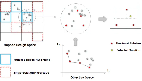
3.4.3 Filtering method ... 46

3.4.4 Navier-Stokes analysis ... 49

3.5 Test case ... 51

3.5.1 Optimization problem formulation ... 52

3.5.3 Results and discussions ... 55

3.6 Conclusion ... 62

3.7 Acknowledgment ... 63

CHAPTER 4 ARTICLE 2: PHYSICS-BASED SURROGATE OPTIMIZATION OF FRANCIS TURBINE RUNNER BLADES, USING MESH ADAPTIVE DIRECT SEARCH AND EVOLUTIONARY ALGORITHMS ... 64

4.1 Abstract ... 64

4.2 Hydraulic turbine design optimization process ... 64

4.3 Multi-fidelity design optimization methodology ... 67

4.3.1 Low-fidelity phase ... 67

4.3.2 Filtering process ... 68

4.3.3 High-fidelity phase ... 68

4.4 Low-fidelity optimization arrangement ... 69

4.4.1 Objective and constraints ... 69

4.4.2 Initial geometry and design variables ... 70

4.4.3 Optimization features ... 71

4.5 Results and discussions ... 73

4.6 Conclusion ... 79

4.7 Acknowledgement ... 80

CHAPTER 5 ARTICLE 3: APPLICATION OF A TERRITORIAL-BASED FILTERING ALGORITHM IN TURBOMACHINERY BLADE DESIGN OPTIMIZATION ... 81

5.1 Abstract ... 81

5.2 Introduction ... 81

5.3 Territorial-Based Filtering Algorithm (TBFA) ... 83

5.3.2 Objective-based filtering ... 84

5.3.3 Space mapping ... 84

5.3.4 Sieving ... 85

5.3.5 Cluster formation ... 86

5.4 Test case 1- hydraulic turbine runner blades ... 87

5.4.1 Low-cost level ... 88

5.4.2 High-cost level ... 90

5.4.3 TBFA functionality and results ... 91

5.5 Test case 2- transonic fan blades ... 96

5.5.1 Aerodynamic shape optimization algorithm ... 96

5.5.2 Blade parameterization, grids and CFD evaluations ... 96

5.5.3 Optimization features ... 97

5.5.4 TBFA functionality and results ... 98

5.5.5 Conclusion ... 101

5.6 Acknowledgment ... 102

CHAPTER 6 GENERAL DISCUSSION ... 103

CHAPTER 7 CONCLUSION AND RECOMMENDATIONS FOR FUTURE WORK ... 108

7.1 Conclusion and contributions of the work ... 108

7.2 Recommendations for future works ... 109

LIST OF TABLES

Table 4.1 : Problem formulation ... 52

Table 4.2 : Optimization scenarios ... 54

Table 4.3 : Independent design parameters and variables ... 55

Table 4.4 : Optimization results ... 59

Table 5.1 : Number of independent parameters & design variables ... 71

Table 5.2 : NOMAD- and EASY-based optimization performances ... 73

Table 5.3 : High-fidelity evaluation results of filtered candidates ... 76

Table 6.1 : Design variables and their bounds ... 88

Table 6.2 : Selected candidates and their performance improvements ... 94

LIST OF FIGURES

Figure 1-1 : Worldwide renewable energy market shares ... 1

Figure 1-2 : Employment factors by renewable energy technologies at the end of 2014 ... 2

Figure 1-3 : Hydraulic turbine application range ... 3

Figure 1-4 : Francis turbine ... 3

Figure 1-5 : Common industrial runner design process ... 4

Figure 1-6: Modification of outer contour and trailing edge positions ... 5

Figure 2-1 : Velocity triangle downstream the runner ... 11

Figure 2-2 : R-Z cross section of a Francis runner ... 12

Figure 2-3 : Turbulence models ... 14

Figure 2-4 : Optimization flowchart ... 17

Figure 2-5 : Pareto front for two objective functions and a decision criterion example ... 18

Figure 2-6 : Computational time comparison of gradient calculation ... 19

Figure 2-7 : Adjoint-based design flowchart ... 19

Figure 2-8 : MADS flowchart ... 21

Figure 2-9 : Mesh shrinkage in a Poll step ... 21

Figure 2-10 : Schematic of an EA loop ... 23

Figure 2-11 : Flowchart of a functional SBO algorithm ... 25

Figure 2-12 : AMMO flowchart ... 28

Figure 2-13 : Illustration of the manifold-mapping model alignment ... 29

Figure 3-1 : Multi-fidelity design optimization algorithm ... 38

Figure 3-2 : Illustration of operating point correction ... 42

Figure 3-3 : Illustration of target correction ... 43

Figure 3-5 : Sieving process; selecting one candidate from each hypercube ... 48

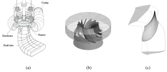
Figure 3-6 : (a) Francis turbine components. (b) Runner flow domain. (c) Single-blade computational domain ... 51

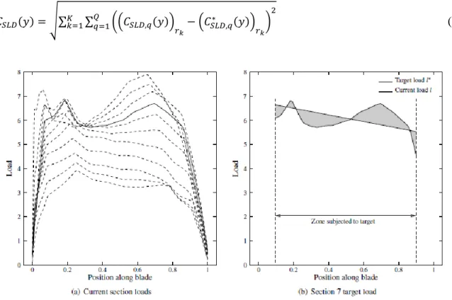
Figure 3-7 : Blade loading: (a) Loading curves of different blade sections. (b) Target load definition based on the section loading curve ... 53

Figure 3-8 : Improvement history of tangential velocity objective function using two optimization scenarios ... 56

Figure 3-9 : (a) Optimization results of A2 and B3 in the objective space. (b) Selected solutions after sieving process. (c) Selected candidates after clustering ... 57

Figure 3-10 : (a) Efficiency curves. (b) Losses of runner and draft tube ... 59

Figure 3-11 : (a) Geometry comparison (white: the original blade, red: B3 optimized blade), (b) Curvature comparison (original blade represented by dashed line) ... 60

Figure 3-12 : Tangential velocity improvement of B3 optimized blade at the targeted BEP ... 61

Figure 3-13 : Blade loading comparison between (a) original blade and (b) B3 optimized blade at new BEP ... 61

Figure 4-1 : Runner design loop interactions ... 66

Figure 4-2 : Multi-fidelity design optimization algorithm ... 67

Figure 4-3 : Initial blade geometry, single-blade and runner flow computational domain ... 70

Figure 4-4 : Blade thickness profile ... 71

Figure 4-5 : Objective value improvement of feasible solutions obtained by NOMAD using different VNS budgets ... 75

Figure 4-6 : Objective value improvement of feasible solutions obtained by EASY using different population sizes and chromosomes lengths ... 75

Figure 4-7 : Comparison of feasible solution distributions in the design space ... 76

Figure 4-8 : Objective value improvement of feasible solutions obtained by the best NOMAD- and EASY optimizations ... 77

Figure 4-9 : Efficiency improvement of the optimized blade versus normalized power coefficient

... 77

Figure 4-10 : Normalized pressure coefficient along the initial blade sections ... 78

Figure 4-11 : Normalized pressure coefficient along the optimized blade sections ... 78

Figure 4-12 : Tangential velocity improvement at the runner outlet; left: base geometry, right: optimized geometry ... 78

Figure 5-1 : Objective-based filtering process: (a) before (b) after filtering. ... 84

Figure 5-2 : Design space mapping process ... 85

Figure 5-3 : Illustration of sieving process; selecting at most one candidate from each hypercube ... 86

Figure 5-4 : Schematic of clustering in a 2-D design space ... 87

Figure 5-5 : Multi-level optimization flowchart ... 88

Figure 5-6 : Schematic of a runner flow passage in R-Z view, with the velocity reference line at the runner downstream ... 90

Figure 5-7 : (a) computational flow domain containing meshed blade surfaces, inlet (top) and outlet (bottom), (b) runner flow computational domain with 13 blades ... 90

Figure 5-8 : Distribution of feasible solutions in the mapped design space, before (a) and after (b) applying the corrected design space ... 91

Figure 5-9 : Distribution of feasible solutions and Pareto front in the objective space, before (a) and after (b) applying the corrected design space ... 92

Figure 5-10 : Selected solutions before the sieving process ... 93

Figure 5-11 : Effect of different sieving grids ... 93

Figure 5-12 : Final candidates selected by clustering unit ... 94

Figure 5-13 : Pressure distribution obtained by potential flow evaluations at OP2 ... 95

Figure 5-15 : Computational domain. Total pressure and total temperature at the inlet, corrected

mass flow at the outlet boundaries ... 97

Figure 5-16 : Feasible solutions and Pareto front in the objective space ... 99

Figure 5-17 : Final candidates selected among sieved solutions ... 99

Figure 5-18 : Correlation of stall margin and efficiency of OP2 ... 100

Figure 5-19 : Distribution of Pareto members and final candidates in the mapped design space 100 Figure 5-20 : Comparison of optimized and reference geometries ... 101

Figure 6-1 : Clustering convergence ... 106

CHAPTER 1

INTRODUCTION

1.1 Hydropower

Due to the depletion of non-renewable fossil energy, the enforcement of the Brazil-Kyoto agreements, and considering the high risk associated with nuclear power plants (especially after Fukushima Daiichi nuclear disaster in 2011), renewable energy markets are projected to continue to grow strongly in the following decades. Among all kinds of sustainable energies, hydropower persists to stand as one of the most important and reliable sources to meet the increasing energy demand. Figure 1-1 shows the portion of renewable energy and hydroelectricity among all energy sources. The global installed hydropower capacity increased from 715 GW to around 1000 GW between 2004 and the end of 2013 [1]. Hydro power had the minimum operation and maintenance labor cost among renewable energy technologies last year (see Figure 1-2).

The global hydroelectric output has always increased. It grew by 2.0% last year, which is below the 10-year average of 3.3% [2]. In spite of this growth, there is a big global potential as well. Norway and Paraguay produce almost all of their electricity (more than 98%) from hydropower resources [3]. Canada constitutes the third-largest generator of hydroelectricity in the world, despite a much smaller population than other key hydro players, China and Brazil. Canada had 77.6 GW installed hydropower capacity at the end of 2014, which accounts for 63% of the country’s power generation. Surprisingly, there is a technical potential of adding 160 GW as well. Having already deployed 38.4 GW, Québec is the fourth-largest producer of hydroelectricity in the world after China, Brazil and the United States, and the largest producer in Canada [4].

Figure 1-2 : Employment factors by renewable energy technologies at the end of 2014 [1]

1.2 Francis turbine

With more than 60% of the global hydroelectric generation, the Francis turbine is the most widely utilized type of turbine in the world. It is also the most commonly used turbine in Canada and Hydro-Québec’s power systems.

James B. Francis developed the Francis turbine in 1848. As a reaction turbine, the pressure of the fluid changes as it passes through the immersed rotor blades. This type of turbine is quite versatile and adaptable to different projects, since its power output ranges from just a few kilowatts up to 1000 MW (see Figure 1-3).

Figure 1-4 shows the main components of a Francis turbine. The spiral casing receives the water, which is transferred from the lake behind the dam via the penstock. The spiral shape of the casing converts the axial flow into radial flow and distributes uniformly the flow into the stay vanes. The guide vanes are simultaneously adjustable and control the inflow characteristics by changing the inlet area (i.e. opening angle) and the angle of attack. The runner is connected to the generator by the shaft axis. It extracts the flow energy and converts the angular momentum of the flow into mechanical momentum. The draft tube recovers most of the flow kinetic energy by converting it into potential energy, which increases the effective head of the turbine.

Figure 1-3 : Hydraulic turbine application range [5]

1.3 Current hydraulic turbine runner design process

In a hydraulic turbine design process, designing the runner is one of the most challenging steps. Runner design has a huge influence on the design of other components. Also, the design of other components, particularly guide vanes and draft tube, affects the runner design. These design interactions are part of the runner design complexity, especially under the consideration of design time limits. The main challenges come from the nature of runner flows. Each runner is unique, since each design project has its own design criteria. To overcome these challenges, the designer needs a solid knowledge of fluid mechanics, as well as a deep understanding and excellent visual imagination of flow behavior inside the runner. He has to take into account different working scenarios and various operating conditions. After taking care of hydraulic design criteria, the designer should consider other disciplines such as structural and manufacturing criteria.

In hydrodynamic design, the designer employs all available evaluation tools, from the cheapest low-fidelity solvers to expensive high-fidelity CFD analyses. Figure 1-5 shows how the hydraulic design network connects the designer to the existing tools. While low-fidelity CFD analyses carry out the major portion of design iterations, high-fidelity CFD solvers evaluate the promising designs mainly in order to verify the main design characteristics and justify final tuning. The designer also uses expensive experimental investigations mostly to validate the final design. In addition, experimental investigations are performed to evaluate very complex phenomena that are difficult to predict with regular CFD tools, such as cavitation.

Parameterization Low-fidelity CFD analysis Experimental validation High-fidelity CFD analysis Many interactions A few interactions Runner designer Several interactions

Figure 1-5 : Common industrial runner design process

Different designers may utilize different parameterization methods in order to play with geometric parameters. They usually spend a lot of time to manipulate the blade curvature and leading and

trailing edge shapes. Trailing edge shape is usually modified by changing the blade length on each blade section. Blade thickness profile is usually corrected later. Inner and outer contours are modified by changing the coordinates of several control points. For example, Figure 1-6 shows changing outer (band-side) contour by playing with cylindrical coordinates of two points on the contour. Also reducing the blade section length produces a shorter blade than the original one (represented by dashed line) by moving the trailing edge towards the upstream.

Figure 1-6: Modification of outer contour and trailing edge positions

The aforementioned points indicate that the runner designer’s experience and intuition play a big role to accomplish this difficult task. This severe dependency causes a lot of designer interactions, which is a drawback considering the duration of the process. Also, the new design concepts may be trapped in a comfort design zone, which is inevitably built by past designer’s experience. In the super-competitive global market, time and cost of the design process are always big concerns. Based on the aforementioned drawbacks of the current design process, these concerns are not properly taken into account in the current design framework.

1.4 Research questions and objectives

The present thesis proposes answers to the following main research questions:

1. How to reduce designer interactions in order to increase the efficiency of the runner design process?

2. How to integrate multi-fidelity runner flow analyses into an automatic design optimization methodology?

3. In the sake of runner performance improvement, what are the objectives and constraints, employed in which optimization configuration?

The aim of this Ph.D. research is to develop a new design methodology that optimizes the geometry of Francis turbine blades, in order to balance time and cost of design, and yield efficient runners, while adhering to different types of design constraints. To reach an efficient optimization methodology, a multi-fidelity framework has been developed, which can take maximum advantage of the low-fidelity model speed and high-fidelity model accuracy.

To effectively develop a design optimization tool, which is practical and reliable for designers, these specific objectives are defined:

1. Develop a multi-fidelity optimization methodology that relies on available industrial resources, e.g. parameterization methods and low- and high-fidelity flow solvers.

2. Investigate different low-fidelity optimization formulations to achieve the expected runner hydrodynamic performance improvement.

3. Demonstrate successful implementation of the proposed methodology and validate it by applying it to different Francis runner optimization problems.

1.5 Thesis overview and work organization

This thesis contains six chapters. Following the above introductory chapter, Chapter 2 provides a literature review of hydraulic turbine evaluation methods, different optimization categories, and surrogate-based multi-fidelity techniques. This chapter also covers the recent progress in hydraulic turbine evaluation and optimization.

Three articles will be presented in Chapters 3 to 5 respectively. They contain all materials presented in the three articles in the thesis format. Although there are some mutual materials in these three articles, they mainly focus on answering the following questions respectively:

1. What is the proper design optimization methodology considering the available runner flow analyses and parameterization tools?

2. In a multi-fidelity optimization methodology, what is the proper derivative-free optimization strategy and what are important optimization features based on characteristics and challenges of the problem at hand?

3. What are the characteristics of an infill method to connect low- and high-fidelity phases together?

Chapter 3 includes the first article entitled “Multi-fidelity shape optimization of hydraulic turbine runner blades using a multi-objective mesh adaptive direct search algorithm”, accepted for publication in the Elsevier journal of Applied Mathematical Modelling. This article proposes the newly developed multi-fidelity design optimization methodology and its components, formulations, and functionality validation through a medium-head Francis turbine runner optimization. This case study also investigates the effect of the number of overall loop iterations with fixed high- and low-fidelity computational budgets. The number of loops determines how often the low-fidelity problem formulation would be corrected as well. In this test case, the BIMADS algorithm handles two velocity objective functions with four constraints. Using two types of design variables represented by up to 17 parameters provides the lowest parameterization flexibility among all test cases.

Chapter 4 presents the second article entitled “Physics-based surrogate optimization of Francis turbine runner blades, employing mesh adaptive direct search and evolutionary algorithms”, published in the International Journal of Fluid Machinery and Systems. This article concentrates on evaluation of different optimization techniques using the MADS and an evolutionary algorithm applied to a low-head Francis runner optimization problem. Since this problem is more challenging than the first one, a new problem formulation is defined using a new objective function and three constraints. In addition, different optimization features are implemented to reach the feasibility and achieve the expected objective improvement. This article indicates the global and local capabilities of two aforementioned optimization algorithms and their advantages for the problem at hand. Chapter 5 contains the third article entitled “Application of a territorial-based filtering algorithm in turbomachinery blade design optimization”, submitted in the Taylor & Francis journal of Engineering Optimization. This article explains the details of the proposed filtering algorithm, which is used as an infill method to choose new design points for costly high-fidelity evaluations. Two different blades are employed that belong to a hydraulic turbine and a transonic fan, in order to demonstrate the method functionality and the influence of important parameters. These two optimization problems utilize different optimization approaches. However, using different

objective functions in two design optimization levels allows us to apply the newly developed filtering algorithm in both problems and investigate its performance.

Among a large number of case studies performed in this project in the field of hydraulic turbines, only several cases have been selected to present in the aforementioned articles. In each article, a completely different Francis runner with different operating conditions is employed. Also various optimization formulations are used with different objective functions and constraints. Beside dissimilar optimization configurations, various design variables with different strategies are used in each article as well.

The sequence of articles shows part of the evolution of runner blade problem formulation. While the first case study presented in the first article applies tangential and meridional velocity objective functions, the second case study only considers tangential velocity as a constraint, and meridional velocity is completely removed from the optimization formulation. Instead, blade average length is taken into account as a new objective. It becomes doable by giving more flexibility to the geometry using more design variables dedicated to the blade length. In addition, three blade loading constraints employed in the first article are replaced with a new one in the next articles.

Chapter 6 provides a general discussion about the results illustrated in the articles and describes briefly their connections. This chapter also demonstrates how the articles complete each other to demonstrate the functionality and performance of the proposed optimization methodology. Finally, Chapter 7 gives the work conclusion and contributions followed by several recommendations for future works.

CHAPTER 2

LITERATURE REVIEW

This chapter only presents the literature most relevant to the research at hand. The first section explains some choices of hydraulic turbine performance evaluations. They can be employed in the optimization methods described in the second section. The third section introduces some surrogate-based optimization methods that can use multi-fidelity evaluations. The fourth section summarizes the chapter.

2.1 Hydraulic turbine performance analyses

In this section several methods of hydraulic turbine flow field analysis are briefly described. It includes the description of several methods ranging from the highest fidelity methods to the lowest ones, with their application cases.

2.1.1 Experimental analysis

Experimental analysis of a hydro turbine is the most accurate methods of flow field investigation that designers use mostly at the final design step. They also use experimental investigations to validate CFD tools. Experimental analysis includes the minimum assumption and the maximum detail of the phenomena. There are some experimental studies of Francis turbines recently cited by researchers are presented below.

Wang et al. [7] studied the unsteady behavior of a prototype 700 MW Francis turbine unit for a 200–700 MW load range with water head of 57m to 90m. They concluded that pressure fluctuations in the draft tube are always stronger than that of upstream flow passages.

Susan-Resiga and Muntean [8] studied the flow characteristics at the outlet of a Francis turbine runner experimentally to investigate the causes of a sudden drop in the draft tube pressure recovery coefficient at a discharge. They used Laser Doppler Velocimetry (LDV) measurements to determine both axial and circumferential velocity components at the runner outlet.

Ciocan et al. [9] analyzed LDV flow survey, pressure and wall friction measurements at the runner outlet using phase average techniques. They aimed to investigate the influence of the rotation and passage of the blade wakes. They also characterized the turbulence and pressure fluctuations.

Tridon et al. [10] focused on the radial velocity components of the swirling flow in a Francis turbine draft tube. Velocity measurements were carried out at CREMHyG (Grenoble) using LDV and PIV1

techniques at four operating points.

The FLINDT project was carried out for a better understanding of flow physics in Francis turbines and to create an extensive experimental database describing a wide range of operating points, which can provide a firm basis for the evaluation of the CFD engineering practice. ALSTOM, Electricite de France, EPFL, General Electric Canada, Va Tech Hydro and Voith Siemens can be mentioned as the main partners of this project. The experimental data are available in several references such as Ref. [11].

Experimental studies are an important part of the designer’s toolbox that can be considered as the highest level of fidelity for turbine performance prediction. However, they cannot be used during the iterative design optimization mainly due to the high cost and time required for these studies.

2.1.2 Mathematical analysis

Due to some simplifying assumptions in the construction of mathematical models, they usually have been categorized as low or medium fidelity models. The main idea is that instead of computing the flow in a certain domain, some algebraic equations can be applied based on operating conditions and kinematic constraints. Thus, runner designers sometimes employ mathematical models to calculate velocity components at a certain operating condition with acceptable accuracy.

Wang and Rusak [12] studied vortex breakdown, and provided a theoretical understanding of swirl flow dynamics. They developed a mathematical model based on the axisymmetric Euler flow. They considered theoretical swirl flow configurations dedicated to a one parameter Batchelor vortex. Leclaire and Sipp [13] did the same investigation with a two-parameter vortex.

Susan-Resiga and co-workers [14] have developed a mathematical model of the swirling flow in Francis turbines for a wide range of operations. They assumed an inviscid steady swirling flow with vanishing radial velocity at the runner outlet. They investigated the correlation between the moment flux of momentum downstream the runner and the operating regime given by the turbine

discharge and head. They represented the relationship between the axial and circumferential velocity components using a swirl-free velocity instead of the traditional relative flow angle at the runner outlet. It has been shown that the swirl-free velocity approach is more suitable to describe the swirl kinematic at the runner outlet. This concept was employed by Kubota et al. [15] to investigate draft tube losses. Kubota and co-workers used a single value corresponding to an arbitrary chosen streamline, and did not consider the axial and circumferential velocity profiles. The swirl-free velocity can be written as:

Vsf = ΩRV2Z / (ΩR-V2ϴ) (2-1)

where V2Z and V2ϴ are axial and circumferential velocities at S2 and Ω is the runner angular speed.

R is the radius measured from the runner axis. Figure 2-1 shows the velocity triangle at the runner downstream (S2 in Figure 2-2). 𝛽2 is the relative flow angle, which was assumed in this research

to depend only on the radius for the section S2.

The main advantage of Susan-Resiga’s model is its ability to compute radial profiles of axial and circumferential velocity components at the runner outlet, without any computation of flow in the turbine. As they have validated the proposed mathematical methodology, it can be used as a low-fidelity solver. By achieving an optimum swirling flow configuration at the runner outlet, the shape of runner blades can be reached through an inverse design approach.

Figure 2-2 : R-Z cross section of a Francis runner [14]

2.1.3 CFD analysis

Since a few decades ago, the table-look up and inflow model approach and expensive experimental studies are being complemented or replaced by Computational Fluid Dynamics (CFD) analyses. CFD tools are usually used to meet the following objectives [16]:

 Understanding details of complex flow behaviors such as cavitation, unsteady vortex shedding, and flow instabilities, which need special modeling due to the phenomenon nature.

 Prediction of hydro turbine performance at design and off-design operating conditions.  Avoiding excessive investigations in the lab and on-site.

 Cost-efficient iterative evaluations required during optimization processes.

Runner designers widely use various CFD analyses to study the flow and evaluate the candidates in different steps of the design process. Basically, CFD tools employ one of the following models:

I) Inviscid flow models:

Inviscid flow models assume an ideal fluid which has no viscosity. Although no practical flow is inviscid, the inviscid flow assumption can be applied when viscous effects can be neglected. For instance, very high Reynolds-number flows such as high-speed external flows around streamlined

bodies (far enough from walls) can be treated as inviscid flows. Since the Reynolds number represents a ratio of convective to diffusive influences, a very high Reynolds number indicates negligible diffusion. Also, the inviscid flow assumption is valid when time scales for diffusion are much larger compared to the time scales for convection. In 2D, the governing equations of such flows are known as the 2D Euler equations:

𝜕𝑈 𝜕𝑡 + 𝑈 𝜕𝑈 𝜕𝑥 + 𝑉 𝜕𝑈 𝜕𝑦 = − 1 𝜌( 𝜕𝑝 𝜕𝑥) (2-2) 𝜕𝑉 𝜕𝑡 + 𝑈 𝜕𝑉 𝜕𝑥+ 𝑉 𝜕𝑉 𝜕𝑦 = − 1 𝜌( 𝜕𝑝 𝜕𝑦) (2-3)

The continuity is integrated in the momentum equation. In these equations, x and y define the Cartesian position, U and V are Cartesian velocity components, p is the static pressure, and 𝜌 is the fluid density.

Potential flow analysis as a low-fidelity method has been applied widely to optimize the shape of hydraulic turbine components. In fact, it is an irrotational Euler flow. One of the best explanations of the potential flow theory is still Holmes and McNabb’s paper [17]. They developed a package of computer programs for the flow analysis through hydraulic turbines. The solution algorithm is a fully three-dimensional Galerkin finite element analysis, using a pre-conditioned conjugate gradient equation solver. Holmes and McNabb applied their program to a Francis turbine runner design to reduce the cavitation problem. They verified the proposed changes of runner in reducing the cavitation and efficiency enhancement in scale models tests and on the full-scale runner. Inviscid analyses can assist the designers to approach quickly the desired targets with very low cost of computation and time. Also, it is one of the most commonly used techniques for the preliminary design step of hydraulic turbine components. For instance, Wu et al. [18] applied inviscid quasi-3D and quasi-3D Euler codes in the preliminary stage of runner optimization.

II) Viscous flow models:

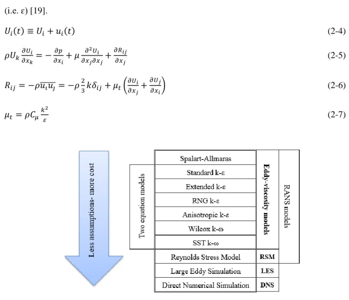
The Navier–Stokes equations describe the motion of viscous fluids. The numerical solution for a turbulent flow is difficult. A proper turbulence model can be chosen based on some criteria that are specific to each problem, such as required physics, time limit and computational resources. Figure 2-3 lists several turbulence models sorted from the simplest to the most complex [19]. Among them, several Reynolds Averaged Navier-Stokes (RANS) models are more common in

hydro turbine applications, which are adaptable and efficient to calculate flow fields. One case of successful applications for each of those models is presented in this part.

RANS models solve Reynolds averaged Navier-Stokes equations (Eq. 2-5), which are based on the decomposition of the quantities into mean and fluctuating terms. For instance, Eq. 2-4 shows the decomposition of the velocity into average (Ui) and fluctuating terms (ui(t)). Time-averaged

statistics of turbulent velocity fluctuations are modeled using functions containing empirical constants and information about the mean flow. RANS models require closure for Reynolds stresses, which is shown in Eq. 2-6. In this equation, μt is the turbulent viscosity. For the k-ɛ model

it is calculated from Eq. 2-7, where 𝐶_𝜇 is a constant turbulent quantity. For instance, in the k-ɛ models, turbulent viscosity is correlated with turbulent kinetic energy, k, and its dissipation rate (i.e. ɛ) [19]. 𝑈_𝑖(𝑡) ≡ 𝑈𝑖+ 𝑢𝑖(𝑡) (2-4) 𝜌𝑈_𝑘𝜕𝑈𝑖 𝜕𝑥𝑘= − 𝜕𝑝 𝜕𝑥𝑖+ 𝜇 𝜕2_𝑈 𝑖 𝜕𝑥𝑗𝜕𝑥𝑗+ 𝜕𝑅𝑖𝑗 𝜕𝑥𝑗 (2-5) 𝑅_𝑖𝑗 = −𝜌𝑢̅̅̅̅̅ = −𝜌_𝑖𝑢_𝑗 2₃𝑘𝛿_𝑖𝑗 + 𝜇_𝑡(𝜕𝑈𝑖 𝜕𝑥𝑗+ 𝜕𝑈_𝑗 𝜕𝑥𝑖) (2-6) 𝜇_𝑡 = 𝜌𝐶_𝜇𝑘_𝜀2 (2-7)

Wu et al. [18] applied a CFD-based design system to a Francis turbine runner and a tandem cascade. They used a standard k-ԑ turbulent flow solver, with special attention paid to flow matching between stationary and rotating parts. Wu and co-workers concluded that 15 blades is an optimal number, due to the compromise between increasing friction loss and flow blockage, and decrease of overall pressure loading per blade by increasing the number of blades. They observed a vortex generated on the pressure side near the leading edge, but it disappeared near the band. The authors indicated that it could be a result of weaknesses of the standard k-ԑ model and wall function to predict swirling and separated flows.

Franco-Nava et al. [20] studied a Francis turbine runner numerically and optimized it based on the genetic algorithm. The Spalart-Allmaras model was used as the turbulence model. To define appropriate inlet flow conditions of the runner, CFD analysis for the wicket gate was carried out too. At the runner outlet, average static pressure was applied based on the experimental data. The authors concluded that the manufacturing and mechanical integrity should be considered in the runner optimization as well.

Hu et al. [21] applied RANS simulations to study the unsteady turbulent flow through Francis turbine components. They used the Renormalization Group (RNG) k-ԑ turbulence model, which was modified in 1986 based on the theory of fuzzy mathematics in order to take into account higher accuracy of prediction of swirling flow influences [22]. Hu and co-workers simulated all components starting from inlet of the spiral casing and ending at the draft tube outlet, using finite volume commercial software, CFX-TASC-flow. Two slip-surfaces were applied between rotating and stationary components, and a mixing surface was applied at the mid-face between the outlet of the guide vanes and the runner inlet.

Yaras and Grosvenor [23] carried out general studies on the axisymmetric separating and swirling flows numerically and experimentally. They evaluated five turbulence models: the k-ԑ model of Chien [24], the two-layer k-ԑ model of Rodi [25], the k-ω model of Wilcox [26], the two-equation Shear-Stress-Transport (SST) model of Menter [27], and the one-equation eddy-viscosity model of Spalart and Allmaras [28]. None of the models used wall-function boundary conditions. They concluded that all models (except Chien’s k-ԑ model) were successful in capturing the surface pressure and skin friction distributions in an axisymmetric separating flow. Also in all cases, a slight over-prediction of static pressure in the separated zone was observed. Menter’s SST model

was the most successful in capturing the velocity profiles, and Rodi’s k-ԑ model was the weakest one in this respect. All models failed to predict the peak k value in the boundary layer. In terms of minimum grid resolution for acceptable prediction accuracy for boundary layer, Rodi’s k-ԑ and Spalart-Allmaras models showed the best performance, requiring a maximum of Yplus=5 and at least 15 nodes within the boundary layer. One of the important conclusions of this research was that all those turbulence models overestimated significantly the radial diffusive transport in the case of strongly swirling confined flow, and SST model yielded the worst prediction.

Susan-Resiga et al. [29] analyzed numerically the swirling flow downstream a Francis runner. They used a simplified straight conical diffuser in order to focus on the decelerated axisymmetric swirling flow in the draft tube cone. They employed a Reynolds Stress Model (RSM) in the commercial code, FLUENT 6.2.16, with a nonequilibrium wall function. The RSM model involves calculation of the individual Reynolds stresses using differential transport equations. They are employed to obtain closure of the Reynolds-averaged momentum equation. Resiga and co-workers concluded that RSM with a quadratic pressure-strain term can predict accurately the flow behavior. They also investigated a flow control technique, which utilized a water jet injected from the runner crown tip along the axis to remove the vortex breakdown at partial load.

Susan-Resiga and co-workers [30] had used Realizable k-ԑ (RKE) before these investigations, to compute the circumferentially averaged swirling flow in the discharge cone of a Francis turbine at low discharge conditions. The RKE model was developed by Shih et al. [31] to provide superior performance for flows involving rotation, boundary layer under strong adverse pressure gradient, separation, and recirculation. This model satisfies certain mathematical constraints on the Reynolds stress, consistent with the physics of the flow.

Large Eddy Simulation (LES) needs a much finer mesh than what RANs-based models need, and is employed to simulate unsteady flow phenomena. For instance, Pacot and co-workers [32] applied LES to simulate rotating stall phenomena in partial load of a pump turbine machine using about 100 million hexahedral elements. Due to the high computational cost, LES has been recently employed in hybrid RANS-LES turbulence models. For instant, Krappel et al. [33] carried out Francis pump turbine flow simulations at part load conditions using a SST-LES turbulent model with two grids containing about 10 and 20 million cells for the whole machine.

2.2 Optimization methods

Optimization methods can be classified into several categories depending on the type of problems and their specifications, such as continuous and discrete, global and local, linear and nonlinear, single-objective and multi-objective optimizations. Also, two categories of optimization algorithm can be distinguished: the gradient-based and non-gradient (derivative-free) methods, which affect strongly the possibility, robustness, required information for the optimization process, cost of optimization, and the solution quality. In engineering optimizations, almost all problems are subject to constraints which divide the design space into feasible and infeasible regions. In this section, those categories that are more relevant to this research are briefly described.

Figure 2-4 shows the general flowchart of an optimization problem, which employs a high-fidelity CFD chain. This chain includes a mesh generator, a viscous flow solver, and a post-processing. Using a high-fidelity CFD solver lonely in turbomachinery shape optimizations is quite time consuming and computationally expensive. For instance, Flores et al. [34] optimized a Francis runner represented by 24 design variables. They employed a high-fidelity CFD flow solver using the SST turbulence model during the optimization. Flores and co-workers reported that they performed 1000 model evaluations; each model was discretized by about 300000 cells. Each computation took about 15 minutes by parallelizing over four processors. Therefore, the overall time was about 250 hours (i.e. more than 10 days).

Initial design Model evaluation Design update Termination condition Optimized design High-fidelity CFD chain Automatic

optimization loop Yes

No

2.2.1 Multi-objective optimization

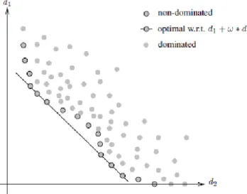
Modern engineering problems usually involve several design objectives and optimal solutions are found as a trade-off among them. In turbomachinery problems dedicated to shape optimization, designers should consider different design aspects (e.g. drag, lift and cavitation). Those objectives may be in conflict and the optimal parameter of one objective usually does not lead to optimality of other objectives. In fact, multi-objective optimization will lead to a set of solutions, called an approximation of Pareto optimal set or Pareto front, which are not dominated by other optimization solutions. Solutions can be chosen after employing additional decision-making criteria (see Figure 2-5).

Figure 2-5 : Pareto front for two objective functions and a decision criterion example

2.2.2 Gradient-based methods

Gradient-based algorithms start from an initial point, and utilize gradient information to decide where to move. Steepest descent and conjugate gradient methods are first-order methods, which typically exhibit linear convergence due to their use of function gradients. The Newton method, as a second-order method, additionally employs the Hessian to reach the minimum. The gradient vector and Hessian matrix can be approximated using finite differences if they are not available analytically, or using adjoint and complex step methods. Figure 2-6 presents a cost comparison of these methods to calculate the gradient vector. In this figure, the time is normalized with respect to the time required for one solution of an aero-structural design [35].

For instance, Tatossian et al. [36] developed an aerodynamic shape optimization approach to improve the performance of hovering rotor blades represented by about 4000 design variables in transonic flow using a discrete adjoint method. Figure 2-7 shows the general design flowchart used in their work. For each design run, 500 multigrid cycles were employed for the flow and adjoint solvers, where each run required between 4 and 7 hours on 12 processors. They performed 25 design cycles to ensure that the minimum had been achieved.

Although gradient-based methods are known as powerful methods for local search, there are some challenges in real problems such as evaluation failures, prohibitive computational cost, and numerical noise that make difficult their systematic use.

Figure 2-6 : Computational time comparison of gradient calculation [35]

2.2.3 Non-gradient-based methods

Many practical applications require the optimization of functions whose gradients are not available or computationally expensive or time consuming to compute. Therefore, various methods have been developed that use the function values at a set of sample points to determine new design points. They can be appropriate algorithms to find different local and global minima in non-convex and discontinuous objective functions as well as discrete spaces. They can also handle noisy objective functions. Non-gradient-based methods are appropriate choices where function evaluations are the results of computer codes, i.e. blackbox, which may fail even for feasible design points. On the other hand, these methods usually require a much larger number of evaluations than gradient-based methods.

Among derivative-free methods, direct-search algorithms (such as MADS [37], Pattern Search [38], and Generalized Pattern Search [39]) have some proofs of convergence to local optimality. In contrast, there are considerable numbers of derivative-free global search methods, such as genetic algorithms [40], evolutionary algorithms [41], particle swarm optimization [42], and simulated annealing [43]. They do not have any optimality convergence guarantee.

Most hydro blade shape optimizations have employed derivative-free optimization techniques [34, 44, 45]. From each aforementioned category (i.e. local and global search derivative-free methods), one optimization method is described in two next following subsections, which have been employed in the present research work.

2.2.4 Direct search algorithms

In direct search algorithms, a set of directions with suitable features are used to generate a finite set of points at which the objective function is evaluated [46]. One of the most recent direct search methods is the Mesh Adaptive Direct Search (MADS) developed by Audet and Dennis [47]. This method is used by NOMAD software employed in case studies presented in this thesis. The MADS algorithm iterates to evaluate blackbox functions at some trial points located on a mesh, to improve the current best solution. The mesh is a discretization of the design space. Figure 2-8 shows the MADS flowchart. Each iteration is composed of two steps: the Search and the Poll.

The Poll generates trial mesh points in certain directions in the vicinity of the best current solution and evaluates those points. When the iteration results in no improvement with respect to objectives and constraints, the next iteration will be initiated on a finer mesh. This algorithmic feature

provides the basis for the convergence analysis of the overall optimization process [48]. Figure 2-9 illustrates an unsuccessful Poll step with mesh refinement. In the first iteration, evaluation of three trial points has not caused function improvement and 𝑥_𝑘 has remained as the best current point. Therefore, new trial points with new directions are set on the refined mesh. The Poll size is directly related to the mesh size and is reduced slower than the mesh size. Therefore, more directions are provided for the new iteration.

Figure 2-8 : MADS flowchart [49]

P6 P5 P4 P3 P1 P2 xk xk ∆k =1/2 ∆k+1 =1/8

The Search step is carried out before the Poll step, which can explore the design space using a surrogate model. The Search can return any point on the underlying mesh in order to improve the current best solution. The default Search step usually uses a quadratic model of all functions by using available evaluations and conducting an optimization on this model. In addition, a variable neighborhood search (VNS) [50] can be employed to escape from local minima.

The MADS algorithm treats constraints in three different ways. The first type of constraints, unrelaxable constraints, cannot be violated by any trial point. In other words, function evaluation will not be considered if at least one of these constraints is violated. For instance, design variable bounds can be treated as unrelaxable constraints. The second type, relaxable constraints, can be violated and the amount of violation is measured. The third type, hidden constraints, is mainly dedicated to blackbox evaluation failures.

The main convergence criterion of the MADS algorithm is met when the mesh size becomes small enough. However, in practice the maximum number of evaluations can be set to stop the optimization with respect to available computational budget. The BIMADS algorithm [51] has been developed to handle bi-objective optimization problems. It solves a series of single-objective sub-problems of the bi-objective problem using the MADS algorithm to obtain an approximation of Pareto front [52].

2.2.5 Evolutionary algorithm

Popular Evolutionary Algorithms (EAs) have been inspired by Darwin's theory of evolution. The EAs are random population-based methods, which are widely used in engineering design due to their robustness and ability to handle single- and multi-objective, constrained optimization problems without getting trapped in local minima [53]. They are also able to obtain Pareto front approximation even after the first run, since in each run all population is evaluated. EAs usually require a large number of function evaluations compared to gradient-based algorithms, which can be their main drawback.

Unlike the MADS algorithm that is relatively new, the first attempts of EAs usage are dated back to the 1950’s, and were performed by Friedberg [54], Bremermann [55], and Box [56]. They initiated the development of three different classes of EAs: evolutionary programming, evolutionary strategies, and genetic algorithms.

EAs handle populations of individuals representing potential solutions, evolving from generation to generation. Each individual is evaluated to calculate the fitness or cost value based on the objective function. Then the EA selects the most fitted individuals among the last generation, called parents, in order to evolve them using evolution operators, recombination (or crossover) and mutation (see Figure 2-10). The new population is called offsprings or children, which is expected to be more adaptable to the environment [57]. In the second article in Chapter 4, EASY employs the aforementioned EA algorithm.

The EAs usually consider constraints by applying penalty functions [58], which significantly decrease the chance to survive for individuals violating the constraints.

Figure 2-10 : Schematic of an EA loop [57]

2.3 Multi-fidelity surrogate-based optimization

High-fidelity investigations are quite accurate, but typically time consuming and expensive. In most industrial optimization problems, it is not preferable to use costly high-fidelity evaluations in the main iterative optimization loop, especially by using demanding derivative-free methods. Therefore, multi-fidelity optimization methodologies have been developed to integrate lower fidelity evaluations in conjunction with the high-fidelity ones, in order to combine their advantages and alleviate their drawbacks. Multi/variable fidelity optimization methods usually have different phases/levels. In the low phase, Surrogate-Based Optimization (SBO) techniques are mostly employed in order to decrease the number of high-fidelity evaluations. In such a framework, a greater quantity of relatively cheap information can be coupled with a small amount of expensive information to increase the accuracy of the surrogate model (if required or possible). It has been

shown that the multi-fidelity SBO methods are more scalable to larger numbers of design variables and much less high-fidelity evaluations are needed to obtain a given accuracy level [49].

Refs. [59-61] have provided comprehensive studies and overviews of different surrogate methods and their implementation in the literature. The surrogates can be created by applying each type of these methodologies, or a combination of them:

1. By using mathematical approximations of the high-fidelity model named functional surrogates.

2. By using a reduced-dimension space.

3. By using reduced physics (e.g. inviscid flow solvers for flow field calculation). In the case of using CFD tools, two more choices will be added:

4. By using variable-resolution models, which means the same high-fidelity solver is used, but with a coarser grid.

5. By using variable-accuracy models, which means the convergence tolerance is reduced in high-fidelity CFD analyses.

Numbers 3 to 5 are also called physics-based surrogates [49].

2.3.1 Functional surrogates

Functional or mathematical surrogates (also called surrogate models) consist of approximation models that mimic the behavior of the simulation model. They are usually constructed based on modeling the response of the simulator to a number of data points, without any particular knowledge of the physical system. Functional surrogate optimization contains three main steps, which can be iteratively interleaved (see Figure 2-11):

1. Selection of initial data points, also called sequential or optimal experimental design 2. Surrogate model construction

3. Surrogate model optimization 4. Surrogate accuracy assessment

To enhance the surrogate model accuracy, some new points should be chosen and evaluated. They are known as infill points, which are described later in Subsection 2.3.4.

Initial design Model evaluation Surrogate model update Termination condition Optimized design High-fidelity CFD chain Automatic

optimization loop _Yes

No

Surrogate model

Surrogate model optimization

Figure 2-11 : Flowchart of a functional SBO algorithm

One of the most widely used forms of surrogate models is the Polynomial Response Surface Model (PRSM). A comprehensive overview of PRSM is presented in Ref [62]. The PRSM consists of a group of mathematical and statistical techniques utilized in the development of a relationship approximated by a low-degree polynomial model, between an interest response and some variables. Radial Basis Functions (RBFs) use a weighted sum of radially symmetric functions to emulate complicated design landscapes. Typical basis functions are linear, cubic, and thin plate spline. Employing parametric basis functions can bring more flexibility (e.g. Gaussian) [60]. For instance, Georgopoulou et al. [63] optimized runner blades of Francis and Kaplan turbines using an RBF in a hierarchical surrogate-based evolutionary algorithm (EA). Earlier, they had shown the role of employing this method in multi-objective EA in mathematical and aerodynamic shape optimization problems [64]. The reported results of Francis runner design after 400 exact evaluations showed no significant improvement of cost functions in comparison with the results of 400 Euler-based evaluations. For Kaplan runner optimization, they carried out 3500 high-fidelity evaluations, which is quite high. It indicates that the developed surrogate-based multi-fidelity design methodology is not efficient enough due to its disability to employ all benefits of low-fidelity and high-fidelity models.

Kriging is another well-known surrogate model named in honor of the South African mining engineer Danie Krige, who developed and applied mathematical statistics in ore evaluations [60,

65]. It constitutes a Gaussian-based modeling method as a particular case of RBF models. Unlike most functional surrogates, Kriging does not assume independent error terms (i.e. residuals). It assumes a correlation between the residuals of two design points related to their spatial distance. Due to its expenses, it is usually used when the true function is computationally expensive, e.g. CFD-based calculation [60]. For instance, Jouhaud et al. [66] applied a Kriging model to optimize a 2D airfoil shape. A low-dimensional model parameterized the geometry, which consisted of two design variables.

The Artificial Neural Network (ANN) method is based on the neuron function. The network is trained by solving a nonlinear least-square regression problem for a set of training points. A typical ANN consists of several layers each including several nodes. The ANN receives the input data from the input layer using input nodes. Then, at least one intermediate or hidden layer contains hidden neurons that stand for computational units. Neuron connections transfer data between different layers. The last layer contains output nodes that deliver the final ANN response [59]. More recently, multi-surrogate techniques have been developed to employ more than one functional surrogates with the same evaluation points. This combination can eliminate the risk of wrong surrogate model selection and provides the robustness to choose the most proper one at each optimization level. For instance, Badhurshah and Samad [67] incorporated PRSM, RBF, and Kriging to optimize a bidirectional impulse turbine blade. The high-fidelity results obtained by RANS simulations were used to train the surrogates and find the optimal points via a hybrid genetic algorithm. They also applied a weighted average surrogate. While multi-surrogate usage was quite satisfactory, the weighted average surrogate did not have the expected performance. Badhurshah and Samad reported a high number of 600 iterations and an average time of 6 hours for a single simulation. Vesting and Bensow [68] employed several ANNs and Kriging models and a combination of them in a marine propeller optimization. They also reported a large number of iterations that were time consuming even with eight parallel computations.

2.3.2 Physics-based surrogates

In the case of a CFD-based optimization, physics-based surrogates use simplified governing equations, coarser discretization grids, or relaxed convergence tolerances, or a combination of them. Unlike functional surrogates, physics-based surrogates cannot be corrected and consequently

their accuracy cannot be improved. However, the optimization problem can be corrected to yield more global accuracy and to approach actual optimal solution points.

Jameson and co-workers employed an adjoint method in a SBO of airfoils, using simplified physics; potential flow [69] and compressible Euler flow [70]. Forrester et al. [71] used partially converged CFD results as physics-based surrogates to build a Kriging approximation. They concluded that partially converged results can produce globally more accurate surrogate models than converged simulations for a given computational budget. In addition, they reported a 48% time saving achieved in a three-dimensional wing problem. Leary et al. [72] also combined physics-based surrogate using coarse grids with functional surrogate using an ANN.

In hydraulic turbine studies, for instance, Wu et al. [18] applied an inviscid flow solver for the first optimization phase of a Francis turbine runner. In the second phase, they employed a RANS model. In fact, they did not apply the high-fidelity solver actively in the optimization process. As a result, according to their reports, the optimized solution is not significantly promising, especially at off-design operating conditions.

2.3.3 SBO management techniques

Solving SBO problems needs managing some optimization aspects, such as the switching scenario between low- and high-fidelity evaluations (e.g. surrogate and high-fidelity CFD evaluations), low- and high-fidelity budgets, low-fidelity optimization or surrogate correction methods, number of design variables and their bounds in different optimization steps. Different SBO management techniques have been developed. A few of them are briefly described in this subsection.

Approximation Model Management Optimization (AMMO) [73] employs a variable fidelity technique using a trust region approach [74]and quadratic approximations. The optimizer receives the objective function and constraint values and their sensitivities from the low-fidelity evaluations. As a first-order optimization method, the response of the low-fidelity model is corrected to satisfy zero- and first-order consistency conditions with the high-fidelity model, which can guarantee the convergence beside trust region usage. To increase the convergence rate of the algorithm, the high- fidelity Hessian can be used to satisfy the second-order consistency. For complicated industrial problems, the Hessian can be replaced with approximation methods (e.g. finite difference); consequently semi-quadratic convergence can be obtained. Figure 2-12 shows the AMMO algorithm flowchart.

For instance, Alexandrov et al. [75] employed this methodology to design a 2D airfoil using RANS and Euler equations respectively for high- and low-fidelity evaluations.

Figure 2-12 : AMMO flowchart [49]

Some SBO techniques do not require sensitivity information. For instance, Efficient Global Optimization (EGO) [65] uses a zero-order optimization strategy employing Bayesian approach along with a Kriging surrogate [76].

The convergent Trust-Region Model Management (TRMM) methodology [77] has been developed for variable-parameterization design methods. This SBO technique uses low-fidelity models and low-fidelity design spaces. Mathematical relations are defined between design vectors by a mapping method, called Space Mapping (SM) [78, 79]. To have an efficient SM optimization algorithm it is really important to have a computationally cheap but sufficiently accurate low-fidelity model. The initial SM techniques were based on a linear correction of the coarse model design space, called input SM [78]. Instead of reshaping the model domain in input SM, the model response can be corrected, called output SM [80], or the overall model properties can be changed, called implicit SM [80]. Manifold mapping (MM) [81] is a particular case of output SM, which can be expected to converge if the model response is smooth. The manifold-mapping model