HAL Id: hal-00779389
https://hal.archives-ouvertes.fr/hal-00779389
Submitted on 22 Jan 2013
HAL is a multi-disciplinary open access
archive for the deposit and dissemination of
sci-entific research documents, whether they are
pub-lished or not. The documents may come from
teaching and research institutions in France or
abroad, or from public or private research centers.
L’archive ouverte pluridisciplinaire HAL, est
destinée au dépôt et à la diffusion de documents
scientifiques de niveau recherche, publiés ou non,
émanant des établissements d’enseignement et de
recherche français ou étrangers, des laboratoires
publics ou privés.
System optimization by multiobjective genetic
algorithms and analysis of the coupling between
variables, constraints and objectives
Jérémi Regnier, Bruno Sareni, Xavier Roboam
To cite this version:
Jérémi Regnier, Bruno Sareni, Xavier Roboam. System optimization by multiobjective genetic
al-gorithms and analysis of the coupling between variables, constraints and objectives. COMPEL: The
International Journal for Computation and Mathematics in Electrical and Electronic Engineering,
Emerald, 2005, vol. 24, pp.805-820. �10.1108/03321640510598157�. �hal-00779389�
System Optimization by Multiobjective Genetic Algorithms and Analysis of the
Coupling between Variables, Constraints and Objectives
J. Régnier, B. Sareni, X. Roboam
Laboratoire d’Electrotechnique et d’Electronique Industrielle UMR INPT-ENSEEIHT/CNRS N°5828,
BP 71 22, 31 071 Toulouse Cedex, France
E-mail : [email protected], [email protected], [email protected]
Abstract : This paper presents a methodology based on Multiobjective Genetic Algorithms (MOGA’s) for the design of electrical engineering systems. MOGA’s allow to optimize multiple heterogeneous criteria in complex systems, but also simplify couplings and sensitivity analysis by determining the evolution of design variables along the Pareto-optimal front. A rather simplified case study dealing with the optimal dimensioning of an inverter – permanent magnet motor – reducer – load association is carried out to demonstrate the interest of the approach.
Keywords : System Design, Multiobjective Optimization, Genetic Algorithms, Coupling Analysis I. INTRODUCTION
The existence of strong coupling levels in complex heterogeneous electrical devices leads to study the system design as a whole. The best architecture and the corresponding dimensioning have to be determined in order to minimize (or maximize) number of performance criteria (global losses, harmonic distortion, masses, economical cost…) with respect to several constraints. The resulting mathematical optimization problem is usually difficult since it involves mixed variables (continuous variables related to the real dimensioning parameters and combinatorial variables associated with architecture characteristics and discrete dimensioning parameters), various constraints and multiple objectives. Using traditional optimization approaches like gradient based methods is not suitable because of these combinatorial features and the difficulty to obtain analytically constraint and objective derivatives in case of numerical simulation. Genetic Algorithms (GA’s) are well suited to treat this kind of problem. Because of their ability to explore multiple solutions in parallel, standard GA’s can be easily extended to solve multiobjective problems and find the set of best trade-offs. This paper illustrates the application of MOGA’s to the optimal design of a “simple” electromechanical system based on an inverter – permanent magnet motor – reducer – load association.
II. MULTIOBJECTIVE OPTIMIZATION WITH GENETIC ALGORITHMS II.1. Multiobjective Optimization Problem and Pareto Optimality
The multiobjective optimization seeks to simultaneously minimize n objectives where each of them is a function of a vector X of m parameters (or design variables). These parameters may also be subject to k inequality constraints, so that the optimization problem may be expressed as :
k i g f f f f i n ... 1 for 0 ) ( subject to )) ( , ), ( ), ( ( ) ( Minimize 1 2 X X X X X (1)
For this kind of problem objectives are typically conflicting with each other. Thus, in most of cases, it is impossible to obtain the global minimum at the same point for all objectives. Therefore, the problem has no single optimal solution but a set of efficient solutions representing the best objective trade-offs. These solutions consist of all design variable vectors for which the corresponding objective vectors cannot be improved in any dimension without degradation in another. They are known as Pareto-optimal solutions in reference to the famous economist [1]. Mathematically, Pareto-optimality can be expressed in terms of Pareto dominance. Consider two vectors X and Y from the design variable space. Then, X is said to dominate Y if and only if [2]-[5] : ) ( ) ( ... 1 and ) ( ) ( ... 1 n fi X fi Y j n fj X fj Y i (2)
All design variable vectors which are not dominated by any other vector of a given set are called non-dominated regarding this set. The design variable vectors that are non-dominated over the entire search space are Pareto-optimal solutions and constitute the Pareto-Pareto-optimal front.
II.2. Multiobjective Optimization Approaches and Decision Making
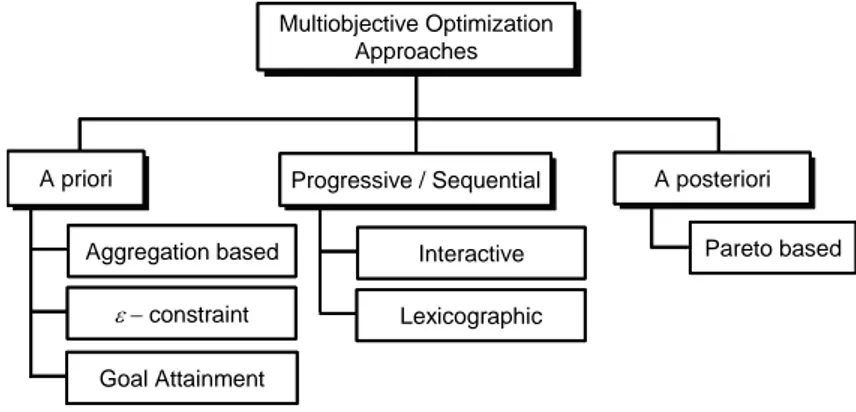
Multiobjective optimization methods aim at finding one or multiple Pareto-optimal solutions to a particular optimization problem. Various multiobjective approaches can be used to guide the Decision Maker towards a final solution among the Pareto-optimal set. A classification of these approaches is depicted in Fig. 1.
Multiobjective Optimization Approaches Multiobjective Optimization Approaches A posteriori A posteriori Goal Attainment constraint Aggregation based A priori
A priori Progressive / SequentialProgressive / Sequential
Lexicographic
Interactive Pareto based
Multiobjective Optimization Approaches Multiobjective Optimization Approaches A posteriori A posteriori Goal Attainment constraint Aggregation based A priori
A priori Progressive / SequentialProgressive / Sequential
Lexicographic
Interactive Pareto based
Figure 1: Classification of Multiobjective Optimization Approaches
We choose to classify Multiobjective Optimization approaches as many researchers [2], [6] defining three variants of the decision making :
A priori approaches (Decide Search) – The Decision Maker combines the differing objectives into a global
quality function. Thus, the multiobjective problem is transformed into a standard scalar optimization problem which can be solved using traditional optimization methods. This approach includes aggregation based methods such as weighting-sum or fuzzy logic techniques, –constraint procedure and goal attainment method. Although they have been widely used in the past, a priori techniques suffer from various drawbacks. In particular, in one optimization run, they provide a single Pareto-optimal solution. Moreover, this investigated Pareto-optimal solution is very sensitive to the scalarization of the objectives and the choice of parameters (e.g. weighting coefficients, target values...) associated with the preferences of the Decision Maker.
Progressive and sequential approaches (Decide Search) – The Optimization Process and the Decision
Making are intertwined. The preferences of the Decision maker are sequentially updated in function of the result of the Optimization Process. Note that a priori approaches can be iteratively used as progressive approaches as well as traditional techniques such as lexicographic method. The main drawback of these approaches resides in the fact that they require multiple optimization runs to provide multiple Pareto-optimal solutions to the Decision Maker.
A posteriori approaches (Search Decide) – These approaches provide in a single optimization run a set of
Pareto-optimal solutions to the Decision Maker who can choose among that set. They essentially include population based optimization methods such as Multiobjective Evolutionary Algorithms (e.g. Genetic Algorithms) [2]-[5] or Multiobjective Particle Swarm Optimizers [7].
II.3. Multiobjective Genetic Algorithms
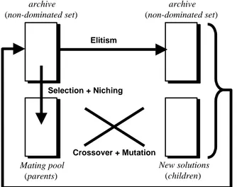
Since the mid-1990s, there has been a growing interest in solving multiobjective problems by Genetic Algorithms. In particular, elitist MOGA’s based on Pareto approaches have become more and more popular because of their capabilities to approximate the set of optimal trade-offs in a single run [2]-[4]. Elitist MOGA’s use an external population, namely archive, which preserves non-dominated individuals in the population. At each generation, individuals (parents) selected from the archive (and/or from the population) following Pareto domination rules (typically expressed by (1)) are crossed and mutated to create new individuals (children). The population of children and the archive are merged to assess the non-dominated set of the next generation. If the number of non-dominated individuals is higher than the size of the archive, a clustering method is used to preserve most representative solutions and eliminate others in order to keep a constant archive size. Note that niching is used in the selection scheme when individuals involved in a tournament have the same Pareto domination rank. The structure of an elitist MOGA is displayed in Fig. 2.
The second version of the Non-dominated Sorting Genetic Algorithm (NSGA-II) [4] is based on the principles previously exposed. NSGA-II determines all successive fronts in the population (the best front corresponding to the non-dominated set). Moreover, a crowding distance is used to estimate the density of solutions surrounding each individual on a given front. In a tournament, if individuals belong to the same front, the selected one is that with the greater crowding distance. This niching index is also used in the clustering operator to uniformly
distribute the individuals on the Pareto front. All details of the algorithm can be found in [4]. Note that some adaptations have been made with the introduction of a self-recombination procedure to increase the robustness of the NSGA-II [8] and by means of an extended Pareto-dominance criterion [10] to include all constraints. In our work, this algorithm is taken as reference for the design of heterogeneous systems in electrical engineering.
archive (non-dominated set) Selection + Niching Mating pool (parents) archive (non-dominated set) Elitism Crossover + Mutation New solutions (children)
Merging (Clustering if necessary)
Figure 2: Structure of an Elitist MOGA (one step generation)
III. OPTIMIZATION AND ANALYSIS OF A SIMPLE ELECTROMECHANICAL SYSTEM III.1. Problem statement and optimization results
To illustrate the use of MOGA’s in electrical engineering, the optimal design of an electromechanical system has been investigated. The corresponding device is based on an inverter–permanent magnet motor–reducer–load association (see Fig. 3).
The purpose is to simultaneously minimize two objectives: the global losses f1(X) and the mass of the system
f2(X). Each objective is composed of partial criteria : f1(X) is the sum of the inverter losses Pinv (switching losses
and conduction losses) and motor losses Pmot (iron and Joule losses) and f2(X) is the sum of the motor mass Mmot
and the inverter heat skin mass Minv. The whole system behavior is described by means of analytical models. All
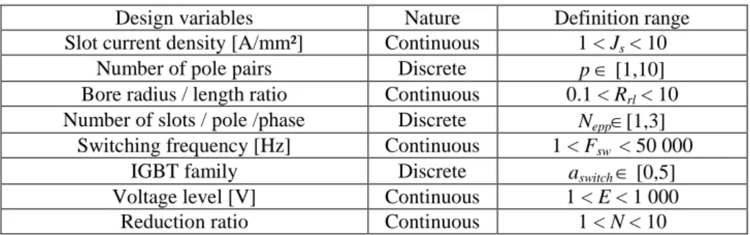
the details dealing with the associated modeling issues can be found in [9]-[11]. The resulting optimization problem can be expressed by (1) with 2 objectives (n=2), 8 design variables (m=8) and 7 constraints (k=7). The design variable vector X and the set of technological and working constraints gk(X) associated to the system are
displayed in Table 1 and 2 respectively. Note that the IGBT family represented by aswitch[0,5] corresponds to
Six Pack modules of IXIS with different range of voltage and current (600V/16A-45A-90A and 1200V/30A-52A-90A). Finally, the whole optimization procedure is displayed in Fig. 4.
The optimization of the system is carried out using the NSGA-II run for 500 generations with a population size of 100. The archive size is also set to 100 individuals and the crossover and mutation rates are respectively 1.0 and 1/m. 10 independent runs are made to take into account the stochastic nature of the GA. The Pareto-optimal front resulting from these runs is displayed in Fig 5. The global losses evolve from 628W to 984W which leads to a global efficiency, in relation to the operating point of the machine (15 kW), varying from 96% to 93.8%. The corresponding system mass is between 94.9 kg and 39.4 kg. The design variables of the boundary solutions shown in Fig. 5 illustrate the diversity of the system configurations along the front.
By providing to the designer a set of optimal solutions, this a posteriori multiobjective approach can help him to understand the main relationships between design variables, constraints, and objectives in the system. In particular, we will illustrated this point in the following sections, through the study of partial objectives, the analysis of couplings, the investigation of parametric sensitivity, and the choice of a final solution in the case of the previously exposed system.
III.2. Partial objective analysis
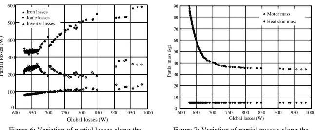
The evolution of the partial objectives along the Pareto-optimal front is displayed in Fig. 6 and Fig. 7. A symmetric variation between iron and joules losses of the permanent magnet machine can be shown in Fig. 6, which illustrates a compensation phenomenon. Concerning the variations of the system mass, we observe in Fig. 7 that the inverter heat skin mass is constant. Its part of the global mass does no exceed 10%. The most significant mass in the system is that of the electrical machine.
~ =
Torque = 100 Nm Speed = 150 rad/s
E : Voltage Level
Rrl : Radius / Length Ratio
JS : Current Density p : Number of pole pairs
Fsw : Switching frequency Heat Skin Weight : IGBT family aswitch Inverter Losses Motor Losses Motor Weight Thermal and Harmonic Distortion Constraints Technological and Thermal Constraints N : Reducer Ratio Smooth pole PMSM analytical model design Smooth pole PMSM analytical model design Inverter model Inverter model Torque-Speed Specifications Torque-Speed Specifications Objective Computing Objective Computing Constraint Computing Constraint Computing Pareto Genetic Algorithm (NSGA-II) Pareto Genetic Algorithm (NSGA-II) N.m 100 load T -1 rad.s 150 load dim T dim N p rl R S J E dim V mot I j P iron P mot M inv P epp N sw F switch a inv M
Figure 3: Electromechanical system design problem Figure 4: Optimization procedure
TABLE I : DESIGN VARIABLES
Design variables Nature Definition range
Slot current density [A/mm²] Continuous 1 < Js < 10
Number of pole pairs Discrete p [1,10]
Bore radius / length ratio Continuous 0.1 < Rrl < 10
Number of slots / pole /phase Discrete Nepp[1,3]
Switching frequency [Hz] Continuous 1 < Fsw < 50 000
IGBT family Discrete aswitch [0,5]
Voltage level [V] Continuous 1 < E < 1 000
Reduction ratio Continuous 1 < N < 10
TABLE II : CONSTRAINTS ASSOCIATED TO THE OPTIMIZATION PROBLEM
g1(X) Minimal number of conductor slots
g2(X) Maximal number of conductor slots
g3(X) Demagnetization magnet limit
g4(X) Maximal winding temperature
g5(X) Voltage supply harmonic distortion
g6(X) Fulfillment of IGBT Voltage range
g7(X) Maximal IGBT junction temperature
600 650 700 750 800 850 900 950 1000 30 40 50 60 70 80 90 100 Global losses (W) S y st e m m a ss ( k g ) -2 A.mm 15 . 2 S J 2 p 637 . 0 rl R Hz 972 sw F 5 switch a V 798 E 1 N -2 A.mm 05 . 5 S J 3 p 1 . 0 rl R Hz 3391 sw F 5 switch a V 624 E 82 . 1 N global losses = 628 W system mass = 94.9 kg global losses = 984.3 W system mass = 39 kg
600 650 700 750 800 850 900 950 1000 0 100 200 300 400 500 600 Global losses (W) Partial los ses (W) Iron losses Joule losses Inverter losses 600 650 700 750 800 850 900 950 1000 0 10 20 30 40 50 60 70 80 90 Global losses (W) P ar ti a l m as s (kg) Motor mass Heat skin mass
Figure 6: Variation of partial losses along the Pareto-optimal front
Figure 7: Variation of partial masses along the Pareto-optimal front
According to these observations, the permanent magnet machine appears as the central element of the system. Indeed, it causes the main mass variations and includes the most important part of the global losses (over 85%). This conclusion was expectable with regard to the complexity of this sub-system which presents some important multi-physical field characteristics.
III.3. Coupling analysis
One of the main difficulties in the system design is to identify couplings between design variables, constraints and objectives in case of a complex multi-physical model. The knowledge of these interactions is valuable with regard to the system behavior understanding. In this context, the global formulation of the problem and the set of solutions obtained with the MOGA allow to characterize and underline these couplings. In order to help the designer in this way, we propose to use two methods : a qualitative graphical analysis of variables along the Pareto-optimal front and an original quantitative method based on correlation coefficients.
A classical coupling analysis can be performed in a graphical way by studying design variable variations of Pareto-optimal solutions in relation to the considered objectives. For example, we show, in Fig. 8 and Fig. 9 a coupling between the number of pole pairs (discrete design variable) and the reducer ratio (continuous design variable) for non-dominated solutions of the Pareto-optimal front. It can be observed that each variation of the number of pole pairs is related to an inverse variation of the reducer ratio. This phenomenon results from the variations of the iron losses in the machine, which are strongly linked to the electrical pulsation pNload of
the motor (iron losses increase when increases). Increasing the number of pole pairs p leads to a growth of which consequently increases iron losses. To avoid an excessive value of iron losses, the reducer ratio N reacts to the increase of p by a simultaneous decrease. Other interesting analysis can be performed by studying different couples of design variables in relation to constraints [9]. This graphical approach is interesting because of its simplicity but it only provides qualitative information about the coupling levels.
Because of this main drawback, we propose to use a correlation coefficient in order to assess quantitatively the influence of couplings. Consider for example two coupled design variables X1 and X2 (see Fig 10). The
correlation coefficient between the corresponding variations of these variables X1 and X1 (see Fig. 11) is
defined by (3) [12]. 600 650 700 750 800 850 900 950 1000 1 1.1 1.2 1.3 1.4 1.5 1.6 1.7 1.8 1.9 2 Global losses (W) R ed u c er r at io 600 650 700 750 800 850 900 950 1000 2 3 4 5 Global losses (W) N u m b er of p ol e p ai rs
Figure 8: Variation of the reducer ratio along the Pareto-optimal front
Figure 9: Variation of the pole pair number along the Pareto-optimal front
1, 2
cov
1, 2
1 2 cor X X X X XX with ) ( 2 ) 1 ( 2 2 ) ( 1 ) 1 ( 1 1 i i i i X X X X X X and i1,...,N1 (3)where N denotes the number of considered points, Xi the standard deviation of Xi, andcov(X1,X2) the
covariance between X1 and X2. Nevertheless, note that this coefficient has no signification with the discrete
design variables. In the example of Fig. 10 and Fig. 11, the correlation coefficient equals –1 which signifies that each variation of X1 is always related to an inverse variation of X2. Therefore, these two design variables are
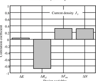
strongly coupled. Fig. 12 presents the correlation coefficients of the current density with the other design variables for Pareto-optimal solutions in the case of the previous investigated system. It shows that the correlation coefficient between the current density Js and the radius/length ratio Rrl of the motor is about –0.9.
Thus, the global system performances are particularly sensitive to these two parameters.Correlation coefficients can also be computed between design variables and partial objectives. For example, Fig. 13 illustrates the correlation coefficients between the current density Js and the partial objectives. In particular, as expected, it can
be observed that Js affects Joule losses Pj (the corresponding correlation coefficient is equal to 0.7) so that an
increase of Js induces an increase of Pj for Pareto-optimal solutions. Similarly, we verify that the inverter losses
strongly depend on the inverter switching frequency since the corresponding correlation coefficient is equal to 0.83. We see here the interest of correlation coefficients which can help the designer to detect the main coupling mechanisms governing the whole system performances.
III.4. Parametric sensitivity analysis
This optimization approach could also be very useful to investigate the influence of parametric variations and especially the restrictions resulting from technological limits on the efficiency of optimal solutions. As an example, we choose to modify the cooling system of the permanent magnet machine (from natural convection to forced ventilation) in order to study the corresponding impact on the global system performances.
0 2 4 6 8 10 12 14 0 5 10 15 20 25 Point V ar ia b le v a lu e 1 X 2 X 0 2 4 6 8 10 12 -10 -8 -6 -4 -2 0 2 4 6 8 10 Variation number V ar ia b le v a ri at io n Xi 2 X 1 X
Figure 10: Evolution example of two coupled design variables X1 and X2
Figure 11: Corresponding variations of the coupled design variables X1 and X2
-1 -0.8 -0.6 -0.4 -0.2 0 0.2 0.4 0.6 0.8 1 Design variables E Δ ΔRrl ΔN C or re la ti on coe ff ic ie nt Current density sw ΔF S J -1 -0.8 -0.6 -0.4 -0.2 0 0.2 0.4 0.6 0.8 1 inv P Pj Piron Mmot C o rr e la ti o n c o e ff ic ie n t Partial objectives Current densityJS
Figure 12 : Example of correlation coefficients between design variables
Figure 13 : Example of correlation coefficients between design variables and partial objectives
Fig 14 shows the comparison between the two Pareto-optimal fronts. The improvement of the cooling system allows to favor the decrease of the system mass. In fact, thanks to the forced ventilation, the size of the motor can be reduced without reaching the thermal limit of the stator winding. The effect of this technological modification can also be observed on the design variables (see Fig. 15). With a natural convection, the reducer ratio N does not exceed 2.2. Even if the increase of N favors the decrease of the motor mass, it involves in the same time an increase of the iron losses and the motor temperature. Therefore, the reducer ratio is limited by the maximum acceptable thermal constraint. The forced ventilation allows to extract more heat from the motor and permits the reducer ratio to grow without an excessive increase of the motor temperature.
III.5. Choice of a final solution
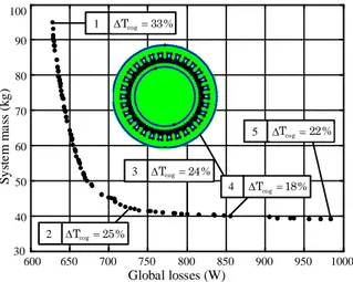
The final choice between all Pareto-optimal configurations can be a posteriori done in relation to other issues which have not been considered in the optimization process. In this paper, we illustrate this point by considering the cogging torque for the final decision.
The cogging torque is computed by using the finite element method from the selected solutions of the Pareto-optimal front. In our example, solution 4 of Fig. 16 presents the lowest value of the cogging torque and can be extracted a posteriori in relation to this added criterion. Note that every solution can be locally optimized by a modification of slot or rotor magnet shape in order to improve the cogging torque value. Once again, the interest of multiobjective a posteriori approaches which provide a set of solutions instead of a single one, has been put forward. Results can be discussed with experts of each sub-system to explore the possible actions to enhance the performance of a particular element and to evaluate with the system designer the impact of the modification on the whole system efficiency.
600 700 800 900 1000 1100 1200 1300 10 20 30 40 50 60 70 80 90 100 Global losses (W) S y st e m m a ss ( k g )
Natural convection cooling Forced ventilation cooling
Thermal constraint on limit
Thermal constraint on limit
600 700 800 900 1000 1100 1200 1300 1 1.5 2 2.5 3 3.5 4 4.5 5 5.5 R e d u c er ra ti o Global losses (W)
Natural convection cooling Forced ventilation cooling
Figure 14 : Influence of the cooling system on Pareto-optimal solutions
Figure 15 : Reducer ratio evolution of the Pareto-optimal solutions with regard to the cooling system
600 650 700 750 800 850 900 950 1000 30 40 50 60 70 80 90 100 Global losses (W) S y st e m m a ss ( k g ) 1 2 3 4 5 % 33 Tcog % 22 Tcog % 18 Tcog % 24 Tcog % 25 Tcog
IV. CONCLUSION
In this paper, we have presented a global approach based on MOGA’s devoted to the design of heterogeneous devices in electrical engineering. It has been shown that MOGA’s are well suited to improve global system efficiency and also to help the designer in the understanding of the relationships between design variables, constraints, and objectives. In particular, from the extraction of Pareto-optimal solutions, MOGA’s facilitate the investigation of parametric sensitivity and the analysis of couplings in the system. For this purpose, we have proposed an original quantitative methodology based on correlation coefficients to characterize the system interactions. Through a simple but typical academic problem dealing with the optimal dimensioning of a inverter – permanent magnet motor – reducer – load association, it has been shown that this multiobjective a posteriori approach could offer interesting outlooks in the global optimization and design of complex heterogeneous systems.
REFERENCES
[1] V. Pareto, Cours d’économie politique, Rouge, Lausanne, Switzerland, 1896.
[2] D.A. Van Veldhuizen. Multiobjective Evolutionary Algorithms: Classifications, Analyses, and New Innovations, PhD thesis, Department of Electrical and Computer Engineering, Air Force Institute of Technology, Wright-Patterson AFB, Ohio, 1999
[3] E. Zitzler, Evolutionary Algorithms for Multiobjective Optimization: Methods and Applications, PhD thesis, Swiss Federal Institute of Technology (ETH), Zurich, Switzerland, 1999J.
[4] K. Deb, S. Agrawal, A. Pratab, T. Meyarivan, "A fast-elitist non-dominated sorting genetic algorithm for multiobjective optimization: NSGA-II", Proceeding of the Parallel Problem Solving from Nature VI Conference, pp. 849-858, 2000.
[5] D.W Corne, J.D Knowles., M.J. Oates, The Pareto Envelope-based Selection Algorithm for Multiobjective Optimization. In M. Schoenauer, K. Deb, G. Rudolph, X. Yao, E. Lutton, J.J. Merelo and H.P. Schwefel eds., Proceedings of the Parallel Problem Solving from
Nature VI Conference, Springer, pp. 839–848, 2000.
[6] Ching-Lai Hwang, Abu Syed Md. Masud, Multiple Objective Decision Making – Methods and Applications, Springer Verlag, 1979. [7] Carlos A. Coello Coello and Maximino Salazar Lechuga. MOPSO: A Proposal for Multiple Objective Particle Swarm Optimization, in Congress on Evolutionary Computation (CEC'2002), Vol. 2, pp. 1051--1056, IEEE Service Center, Piscataway, New Jersey, May 2002. [8] B. Sareni, J. Régnier, X. Roboam, "Recombination and Self-adaptation in Multi-objective Genetic Algorithms", Lecture Notes In
Computer Science, Vol. 2936, P. Liardet et al Eds, pp. 115-126, Springer Verlag, 2004.
[9] J. Régnier, Conception de systèmes hétérogènes en Génie Electrique par optimisation évolutionnaire multicritère, Thèse de Doctorat, n°2006, Institut National Polytechnique de Toulouse, 2003
[10] J. Régnier, B. Sareni, X. Roboam, "Optimal design of electrical engineering systems using Pareto Genetic Algorithms", 10th European
Conference on Power Electronics and Applications, Toulouse, 2003
[11] G. Slemon, X. Liu, "Modeling and design optimization of permanent magnet motors", Electrical Machines and Power Systems, Vol. 20, pp. 71-92, 1992.