LOCAL VISUAL FEATURES EXTRACTION FROM TEXTURE+DEPTH CONTENT BASED ON DEPTH IMAGE ANALYSIS

HAL Id: hal-01082629

https://hal.archives-ouvertes.fr/hal-01082629

Submitted on 13 Nov 2014

HAL is a multi-disciplinary open access

archive for the deposit and dissemination of

sci-entific research documents, whether they are

pub-lished or not. The documents may come from

teaching and research institutions in France or

abroad, or from public or private research centers.

L’archive ouverte pluridisciplinaire HAL, est

destinée au dépôt et à la diffusion de documents

scientifiques de niveau recherche, publiés ou non,

émanant des établissements d’enseignement et de

recherche français ou étrangers, des laboratoires

publics ou privés.

LOCAL VISUAL FEATURES EXTRACTION FROM

TEXTURE+DEPTH CONTENT BASED ON DEPTH

IMAGE ANALYSIS

Maxim Karpushin, Giuseppe Valenzise, Frédéric Dufaux

To cite this version:

Maxim Karpushin, Giuseppe Valenzise, Frédéric Dufaux. LOCAL VISUAL FEATURES

EXTRAC-TION FROM TEXTURE+DEPTH CONTENT BASED ON DEPTH IMAGE ANALYSIS. ICIP

2014, Oct 2014, Paris, France. �hal-01082629�

LOCAL VISUAL FEATURES EXTRACTION FROM TEXTURE+DEPTH CONTENT BASED

ON DEPTH IMAGE ANALYSIS

Maxim Karpushin, Giuseppe Valenzise, Fr´ed´eric Dufaux

Institut Mines-T´el´ecom; T´el´ecom ParisTech; CNRS LTCI

ABSTRACT

With the increasing availability of low-cost – yet precise – depth cameras, “texture+depth” content has become more and more pop-ular in several computer vision and 3D rendering tasks. Indeed, depth images bring enriched geometrical information about the scene which would be hard and often impossible to estimate from conventional texture pictures. In this paper, we investigate how the geometric information provided by depth data can be employed to improve the stability of local visual features under a large spectrum of viewpoint changes. Specifically, we leverage depth information to derive local projective transformations and compute descriptor patches from the texture image. Since the proposed approach may be used with any blob detector, it can be seamlessly integrated into the processing chain of state-of-the-art visual features such as SIFT. Our experiments show that a geometry-aware feature extraction can bring advantages in terms of descriptor distinctiveness with respect to state-of-the-art scale and affine-invariant approaches.

Index Terms—Local visual features; texture+depth; viewpoint invariance

1. INTRODUCTION

Local visual features aim at representing distinctive image details, and are a convenient way to match different instances of the same or very similar content. To this end, local features extraction mimics in a certain way the cognitive behavior of the human visual system (HVS), by first detecting stable and reproducible interest points in the pictures, and then describing the local patches around those key-points. This approach has led to the development of several exam-ples of local features, such as SIFT [1], SURF [2], or binary visual features [3][4][5], which offer various degrees of invariance to trans-lations, scale changes, viewpoint position and illumination changes. Local features extracted from conventional images describe only the photometric content of the scene (given by its projection on the cam-era plane). However, this information is complemented in the HVS by a larger class of stimuli which provide geometrical information about the depth and the relative position of objects in the scene, such as binocular vision, relative size, perspective, motion parallax, etc. [6].

Geometry is fully described through 3D models, such as point clouds and meshes. However, these representations are difficult to acquire and store. Recently, the increasing availability of low-cost depth cameras (such as Microsoft Kinect) has enabled on-the-fly ac-quisition of scene depth along with traditional texture. Differently from 3D models, “2.5D” (texture+depth) content is easier to repre-sent and code [7]. As the quality of the captured depth increases, this information becomes a valuable tool for image analysis and descrip-tion. Nevertheless, very little work has been done so far to extend 2D descriptors when associated depth is available.

This work is one step in the development of such descriptors. To showcase the benefits of using depth in the feature extraction process, we consider a well-known critical issue of 2D local fea-tures: the invariance to viewpoint change. Most state-of-the-art vi-sual features, including SIFT, are designed to be invariant to in-plane rotations. Instead, out-of-plane rotations, i.e., around an axis that does not pass through the optical center, are much more difficult to deal with for two reasons: i) the visual information contained in the projected images is not necessarily entirely preserved because of eventual occlusions/disocclusions; and ii) significant geometrical deformations prevent reliable descriptor matching. In this paper we propose an extension to conventional 2D visual feature computation algorithms aimed at reliable matching across images taken from dif-ferent viewpoints. We assume that the scene depth map is available, e.g., through a depth camera or through sufficiently accurate stereo matching. First, we estimate local approximating planes to objects’ surfaces on the depth image, in correspondence to interest points found in the texture. Then, we use the approximated local normal vector computed from depth to find a normalizing transformation to obtain a slant-invariant texture patch. Since our normalization op-erates between keypoint detection and descriptor extraction, the pro-posed method can be seamlessly included in the processing chain of several 2D local features. In our experiments, we consider the widely used SIFT features as comparison, and we show that depth enables to improve the geometrical consistency of matches, i.e., the ratio of matched pairs of visual features covering the same area of the scene in different views increases significantly. More importantly, the pro-posed normalization renders feature descriptors more distinctive for a wide range of viewpoint changes.

The rest of the paper is organized as follows. Related work is presented in Section 2, the proposed method is described in Section 3, while experiments and test results are discussed in Section 4. Fi-nally, Section 5 concludes the paper.

2. RELATED WORK

The role of geometry in local content description has been known for long time in the field of 3D shape search and retrieval. However, very little has been done when geometry is given under the form of depth. Lo and Siebert [8] apply a SIFT-based descriptor to range (depth) images, in the context of face recognition. There, one important challenge is the ability to recognize faces under varying illumina-tion condiillumina-tions and viewpoint changes. The authors estimate the 3D keypoint orientation using depth map Gaussian derivatives, and use it to select a local sampling frame for the descriptor computation in each point. The resulting descriptors are stable under viewpoint and illumination changes. However, these features are not exactly 2.5D, as no texture data is used. A similar pocedure of normal-based local frame normalization makes part of NARF (Normal Aligned Radial Feature) descriptor presented in [9]. Differently from [8] and [9],

we employ detectors based on texture, and we use depth to normal-ize the corresponding description patches.

A family of techniques addressing significant out-of-plane rota-tions is based on affine region normalizarota-tions. Local affine transfor-mations allow to compensate the geometrical defortransfor-mations produced by significant viewpoint position changes, and have been largely em-ployed in the context of wide baseline stereo matching [10, 11, 12]. Up to the evaluations [13, 14] of such detectors, the best performing techniques are the Maximally Stable Extremal Regions (MSER) [12], Harris-Affine[15] and Hessian-Affine[13] detectors. The MSER de-tector analyzes sequences of nested connected components having contrast border (i.e., a border entirely brighter or darker than any pixel of the component), and selects the ones that minimize a func-tional defined on such sequences. Harris-Affine and Hessian-Affine detectors are based on an iterative procedure that estimates elliptical affine regions for an initial keypoint set, using second-order moment matrix [16]. The affine-covariant detectors may be less repeatable under moderate viewpoint angle changes (up to 40°) [1]. On the other hand, SIFT gives acceptable performance in these cases [17]. Thus, if the viewpoint variation spectrum is not known a priori, affine-invariant features will not necessarily perform better than the conventional visual features.

As an alternative approach to viewpoint invariance, Morel and Yu propose a fully affine invariant technique that simulates affine parameters instead of normalizing them. Their affine-SIFT (ASIFT) technique [17] applies the original SIFT detector-descriptor pair on a set of images rendered from the original one by applying affine transformations. The main drawback of this approach is that it does not allow the extraction of a compact feature set separately from the image, as the raw feature set containing all the descrip-tors from all the transformed images is very large and carries many a priori irrelevant features. This hinders the applicability of this method in image classification and retrieval schemes that work on large datasets of features, such as the bag-of-visual-words [18] or VLAD [19] paradigms. Similarly to ASIFT, an affine-invariant generalization of SURF has been proposed in [20].

3. SLANT NORMALIZATION BASED ON DEPTH The proposed slant normalization approach integrates the conven-tional feature detector/descriptor pair architecture, which is com-posed of the following steps (the items in bold are those affected by slant normalization, which employs depth information):

1. Keypoint detection in the texture image;

2. Local planar keypoint regions approximation and filter-ing of unstable keypoints;

3. Slant normalization of texture image patches; 4. Descriptor computation.

Notice that slant normalization is performed independently of any specific detector/descriptor pair used for steps 1 and 4. Thus, in the following we only discuss steps 2 and 3 in detail.

3.1. Estimation of local approximating planes and keypoint fil-tering

In order to perform slant normalization, the normal to the texture sur-face at each keypoint detected in the texture has to be estimated ro-bustly. Clearly, this cannot be done on texture only and requires 3D information provided by depth. In [8], depth first-order derivatives are used to estimate surface normal vectors. However, this approach

can be imprecise due to the fact that quantized depth maps are often piecewise constant. Moreover, differential characteristics are known to be more prone to noise. Instead, we apply a parametric approach based on locally approximating the surface around the keypoint with a plane.

More formally, let d(i, j) be the depth value in the pixel (i, j), (i0, j0) the keypoint coordinates, S the keypoint area determined

as a function of its scale. We approximate the depth map re-gion corresponding to a keypoint area with the bilinear function

fA,B,C(x, y) = A(x − i0) + B(y − j0) + C. The normal vector

of the plane, n = [A, B, C] is obtained by minimizing the average fitting error

F(A, B, C) = X

(i,j)∈S

|fA,B,C(i, j) − d(i, j)|2, (1)

which can be efficiently solved by least squares.

The robust estimation of the normal vectors may be subject to estimation errors. Thus, we aim to detect those keypoints whose normal is likely to have been poorly estimated, and fil-ter them out from the set of infil-terest points in the texture image. First, we filter keypoints based on the maximum plane fitting error ρ = maxS|fA,B,C(i, j) − d(i, j)|. We keep the keypoints that

satisfy the condition:

ρ < Tmin

S d(i, j). (2)

It is convenient to avoid an absolute threshold in (2), since the dy-namic range of the depth map may be arbitrary (depending on the unit value and the content). Instead the ratio between ρ and min-imum depth value in the keypoint area S does not depend on the dynamic range of the depth map. If this ratio is lower than T , the keypoint is accepted. Moreover, we consider the minimum depth value to take into account the effects of parallax changes according to the distance from the camera – even important viewpoint changes can be approximated by simple shift for background details, whereas near objects undergo more complex perspective transformations. We found out experimentally that the value of T= 0.01 achieves better performance in most cases.

As a second filtering strategy, we reject surfaces with large slant angle, i.e., the angle between the normal and the optical axis of the camera. More precisely, we compute the slant angle as:

θ= arctanpA2_{+ B}2 ₍₃₎

and reject keypoints with θ >80°. The rationale is that these sur-faces, when viewed at large angles, might produce sampling artifacts during the slant normalization phase.

3.2. Local surface sampling and slant normalization

For each geometrically-filtered texture image keypoint, we build a square regular sampling grid window on the approximating plane Ax_{+ By − z + C = 0. More specifically:}

• The center point of the window corresponds to the pixel (i0, j0) projected on the approximating plane.

• The window size is computed as a function of the initial key-point scale σ, slant angle θ and the descriptor patch size, in such a way that the quadrilateral area obtained by the window boundary projection on the camera plane covers the keypoint area in the texture image.

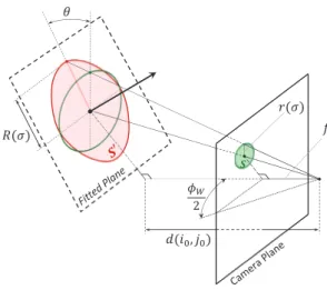
Fig. 1. Estimation of the sampling window size R(σ) in the local approximating plane, obtained from descriptor patch size r(σ). The corresponding keypoint area S′

on the fitted plane is covered by a regular sampling grid which is then projected on the camera plane. The projected grid size is such that it covers the texture keypoint area S.

• The orientation of the sampling window in the plane can be arbitrarily chosen, since the orientation of the texture key-point has to be estimated after slant normalization.

As for the sampling window size, if R(σ) represents the de-scriptor patch size projected on the approximating plane, we choose a square of side M= 2R(σ) spatial units. In turn, if r(σ) is the de-scriptor patch size on the screen and f is camera focal length (both in pixels), it is straightforward to figure out using triangular similarity that

Rcos θ : r(σ) = d(i0, j0) : f. (4)

Having W_2f = tanφW

2 , where W is image width in pixels, φW

is horizontal angle of view of the camera, we get expression of R(σ): R(σ) = 2r(σ)d(i0, j0)

Wcos θ tan φW

2 . (5) Finally, we compute a rectangular grid in the sampling window which is then projected from the local approximating plane to the camera plane. The grid points are distributed regularly in the win-dow, i.e. with an equal step in spatial units. Then we apply the perspective projection model in order to compute grid points posi-tions in pixels. This yields a warped, slant-invariant sampling grid used to sample a patch in the texture image, over which we can com-pute a local descriptor (such as the histogram of gradients used by SIFT). Figure 1 illustrates how the window sampling is built in the approximating plane, and how the correct window size is found.

4. EXPERIMENTS

We tested our approach with the SIFT detector-descriptor, imple-mented in the VLFeat library1. The comparison is performed with classical SIFT features [1] and iterative affine normalization2_,

orig-inally proposed for Harris-Affine detector [15]. We initialize the

it-1_{http://www.vlfeat.org/, we used ver. 0.9.17.}

2_{See VLFeat vl covdet function documentation for details.}

Fig. 2. Examples of images from test sequences (Arnold, 25 images, Bricks, 20 images, Fish, 25 images, Graffiti, 25 images). Graffiti sequence is synthesized from the frontal view of the original Graffiti sequence [14]. The resolution of the images is 960×540.

erative procedure using SIFT detector, i.e., we use for all the test methods the same difference-of-gaussian detector.

For our test we synthesized several image sequences of texture images with associated depth images (few examples are presented in Figure 2). Each sequence is obtained by rendering the same 3D scene from different viewpoints. In each scene the camera was fo-cused at a fixed 3D point, moving along a circular arc. Camera positions and orientation matrices, as well as camera optic system parameters (angle of view used in eq. 5) are provided.

We kept the default parameters proposed in the VLFeat imple-mentation for all the methods. Thus, the descriptor is computed in a square patch of size_{12σ × 12σ pixels}3_{, i.e., we set r(σ) = 6}√_2σ,

which is the bounding circle radius. In a consistent way, for affine elliptical regions we specified the same patch extent.2 The keypoint scale on the transformed patch is based on the initial keypoint scale and computed in a similar way to that presented in Figure 1. How-ever, it is possible to apply an automatic scale selection (e.g., [21]).

The evaluation consists in comparing descriptor sets extracted from a pair of images of a given sequence. To filter out incorrect matches, we compute the overlap error proposed in [14] between corresponding circular/elliptical regions that fit the descriptor patch. As the transformation between a pair in our case is not an homogra-phy (as in Graffiti and Wall sequences in [14]), in order to compute the overlap we sample each keypoint area and reproject the samples from one image of the pair being tested to another one. The camera positions, orientation matrices and depth images are used to com-pute corresponding 3D positions of samples which are then repro-jected to another camera plane. Finally the intersection of the areas is estimated by counting the number of samples fallen into the target elliptical area. We set the overlap error threshold value ǫ0equal to

50%.

We compute the matching score, defined as the number of cor-rect matches divided by the minimum total number of features for the two images [14]. The results are presented for two contents in Table 1. This characteristic evaluates jointly both detector and de-scriptor and depends strongly on the content. Results for standard SIFT features (without normalization), our approach and affine nor-malized features are referred to as Raw, 3D and Aff., respectively. As the matching score may depend more on the keypoint repeatability than on the descriptor performances, for the same detector we ob-tain comparable values between all the methods in all the sequences.

Rotation Fish Graffiti angle, ° Raw 3D Aff. Raw 3D Aff.

5 77.9 78.8 75.0 81.8 79.9 80.5 10 65.5 70.9 64.2 74.3 70.1 73.8 20 50.0 56.2 52.0 60.3 49.6 60.2 30 37.8 52.1 44.2 47.8 39.1 53.0 45 32.4 46.4 37.7 37.4 34.2 47.6 60 31.1 44.0 39.1 31.0 27.7 43.2 90 28.8 36.8 28.5 33.1 31.6 41.6 120 9.8 16.3 12.6 32.8 31.4 37.2 Cmax 433 360 606 643 635 859 Cmin 52 62 94 243 220 397

Table 1. Matching score and number of correct matches C. We present also maximal (Cmax) and minimal (Cmin) numbers of

cor-rect matches (for 5° and 120° rotations). Typically C decreases al-most monotonically as the angle increases.

For sequences with complex geometry of the content, i.e., contain-ing some smooth convex surfaces (Arnold, Fish, Bricks) our method gives the best matching score for the whole rotation angle spectrum. In case of simpler geometry and detailed texture (Graffiti sequence, containing a single plane), the best matching score is achieved by the affine normalization. Our method gives worse results on this se-quence mainly due to cross-matching of texture details that are small and/or have low contrast to the surround. In this case the transfor-mations we apply to sample the descriptor patch may make the un-derlying visual content indistinguishable. The absolute number of correct matches (as well as the overall number of features) obtained with our approach is always lower than the one given by SIFT, as we perform the keypoint filtering before the descriptor computation.

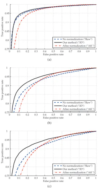
In order to evaluate the advantages of using depth for improving the descriptor distinctiveness, we trace receiving operating charac-teristic (ROC) curves in Figure 3. We estimated ROC jointly on all the sequences (95 images) for three rotation angle ranges: small (up to 30°), medium (30°–60°) and large ones (greater than 60°). We selected randomly at least 15k correct and 15k incorrect matches for each angle range. For standard SIFT features and our approach the ROC is computed as a function of the closest-to-next-closest descrip-tor distances ratio [1], whereas affine normalization performs better when the classification decision is based on the absolute distance to the closest match.

In terms of ROC our method achieves better performance in all the cases except the smallest angles where the original SIFT features performance is generally recognized to be acceptable. The original SIFT is outperformed as it has no normalization to viewpoint angle changes, and the geometrical distortions has a direct effect on the descriptor.

5. CONCLUSION AND FUTURE WORK

In this work we investigate the use of depth information to comple-ment 2D visual features extraction. As an illustration of this concept we proposed a method of local descriptor patch normalization based on scene depth map analysis, targeted to improving visual features stability under a large spectrum of viewpoint angle changes. Our approach presents an alternative to a family of approaches based on the affine normalization in cases when the associated depth image is available. It is designed to be used within any conventional keypoint detector and feature descriptor.

0 0.1 0.2 0.3 0.4 0.5 0.6 0.7 0.8 0.9 1 0.75 0.8 0.85 0.9 0.95 1

False positive rate

True positive rate

No normalization ("Raw") Our method ("3D") Afine normalization ("Aff.")

(a) 0 0.1 0.2 0.3 0.4 0.5 0.6 0.7 0.8 0.9 1 0.75 0.8 0.85 0.9 0.95 1

False positive rate

True positive rate

No normalization ("Raw") Our method ("3D") Afine normalization ("Aff.")

(b) 0 0.1 0.2 0.3 0.4 0.5 0.6 0.7 0.8 0.9 1 0.75 0.8 0.85 0.9 0.95 1

False positive rate

True positive rate

No normalization ("Raw") Our method ("3D") Afine normalization ("Aff.")

(c)

Fig. 3. ROC curves for different rotation ranges: (a) up to 30°, (b) 30° – 60°, (c) greater than 60°.

As we do not make use of the depth image in the keypoint de-tection stage, the detector becomes the weakest point of the entire system. For this reason the achieved performance in terms of the matching score may be limited, especially in case of detailed tex-ture and a relatively simple scene geometry. Thus the primary goal for the future work is to understand how to use the geometry infor-mation provided by depth to improve the keypoint detectors and the determination of their scale on a normalized patch.

6. REFERENCES

[1] D. G. Lowe, “Distinctive image features from scale-invariant keypoints,” International journal of computer vision, vol. 60, no. 2, pp. 91–110, 2004.

robust features (SURF),” Computer vision and image under-standing, vol. 110, no. 3, pp. 346–359, 2008.

[3] S. Leutenegger, M. Chli, and R. Y. Siegwart, “BRISK: Bi-nary robust invariant scalable keypoints,” in IEEE Interna-tional Conference on Computer Vision (ICCV), 2011. IEEE, 2011, pp. 2548–2555.

[4] E. Rublee, V. Rabaud, K. Konolige, and G. Bradski, “ORB: an efficient alternative to SIFT or SURF,” in IEEE International Conference on Computer Vision, 2011. IEEE, 2011, pp. 2564– 2571.

[5] A. Alahi, R. Ortiz, and P. Vandergheynst, “FREAK: Fast retina keypoint,” in IEEE Conference on Computer Vision and Pat-tern Recognition (CVPR), 2012. IEEE, 2012, pp. 510–517. [6] J. Cutting and P. Vishton, “Perceiving layout and knowing

dis-tances: The integration, relative potency, and contextual use of different information about depth,” Perception of space and motion, vol. 5, pp. 69–117, 2010.

[7] P. Merkle, A. Smolic, K. Muller, and T. Wiegand, “Multi-view video plus depth representation and coding,” in Proceedings of the International Conference on Image Processing, vol. 1, Sept 2007, pp. 201–204.

[8] T.-W. R. Lo and J. P. Siebert, “Local feature extraction and matching on range images: 2.5D SIFT,” Computer Vision and Image Understanding, vol. 113, no. 12, pp. 1235–1250, 2009. [9] B. Steder, R. B. Rusu, K. Konolige, and W. Burgard, “Point

feature extraction on 3d range scans taking into account ob-ject boundaries,” in 2011 IEEE International Conference on Robotics and automation (ICRA). IEEE, 2011, pp. 2601– 2608.

[10] A. Baumberg, “Reliable feature matching across widely sep-arated views,” in IEEE Conference on Computer Vision and Pattern Recognition, 2000. Proceedings., vol. 1. IEEE, 2000, pp. 774–781.

[11] T. Tuytelaars and L. J. Van Gool, “Wide baseline stereo match-ing based on local, affinely invariant regions.” in BMVC, vol. 412, 2000.

[12] J. Matas, O. Chum, M. Urban, and T. Pajdla, “Robust wide-baseline stereo from maximally stable extremal regions,” Im-age and vision computing, vol. 22, no. 10, pp. 761–767, 2004. [13] K. Mikolajczyk, C. Schmid et al., “Comparison of affine-invariant local detectors and descriptors,” in Proc. European Signal Processing Conf, 2004.

[14] K. Mikolajczyk, T. Tuytelaars, C. Schmid, A. Zisserman, J. Matas, F. Schaffalitzky, T. Kadir, and L. Van Gool, “A com-parison of affine region detectors,” International journal of computer vision, vol. 65, no. 1-2, pp. 43–72, 2005.

[15] K. Mikolajczyk and C. Schmid, “An affine invariant interest point detector,” in Computer VisionECCV 2002. Springer, 2002, pp. 128–142.

[16] T. Lindeberg and J. G˚arding, “Shape-adapted smoothing in es-timation of 3-d shape cues from affine deformations of local 2-d brightness structure,” Image and vision computing, vol. 15, no. 6, pp. 415–434, 1997.

[17] J.-M. Morel and G. Yu, “ASIFT: A new framework for fully affine invariant image comparison,” SIAM Journal on Imaging Sciences, vol. 2, no. 2, pp. 438–469, 2009.

[18] J. Sivic and A. Zisserman, “Video google: A text retrieval approach to object matching in videos,” in Ninth IEEE Inter-national Conference on Computer Vision, 2003. Proceedings. IEEE, 2003, pp. 1470–1477.

[19] H. J´egou, M. Douze, C. Schmid, and P. P´erez, “Aggregating local descriptors into a compact image representation,” in 2010 IEEE Conference on Computer Vision and Pattern Recognition (CVPR). IEEE, 2010, pp. 3304–3311.

[20] Y. Pang, W. Li, Y. Yuan, and J. Pan, “Fully affine invariant SURF for image matching,” Neurocomputing, vol. 85, pp. 6– 10, 2012.

[21] T. Lindeberg, “Feature detection with automatic scale selec-tion,” International journal of computer vision, vol. 30, no. 2, pp. 79–116, 1998.