HAL Id: hal-01757396
https://hal.archives-ouvertes.fr/hal-01757396
Submitted on 12 Apr 2018
HAL is a multi-disciplinary open access
archive for the deposit and dissemination of
sci-entific research documents, whether they are
pub-lished or not. The documents may come from
teaching and research institutions in France or
abroad, or from public or private research centers.
L’archive ouverte pluridisciplinaire HAL, est
destinée au dépôt et à la diffusion de documents
scientifiques de niveau recherche, publiés ou non,
émanant des établissements d’enseignement et de
recherche français ou étrangers, des laboratoires
publics ou privés.
Development of a falling body viscosimeter for high
pressure measurements
Brice Calvignac, Pauline Vitoux, Élisabeth Rodier, Jean-jacques Letourneau,
Cyril Aymonier, Jacques Fages
To cite this version:
Brice Calvignac, Pauline Vitoux, Élisabeth Rodier, Jean-jacques Letourneau, Cyril Aymonier, et al..
Development of a falling body viscosimeter for high pressure measurements. ISSF 2009 -9th
Interna-tional Symposium on Supercritical Fluids, InternaInterna-tional Society for the Advancement of Supercritical
Fluids ISASF, May 2009, Arcachon, France. 6 p. �hal-01757396�
9th International Symposium on SuperCritical Fluids 2009
18-20 June 2009 - Arcachon (France)
DEVELOPMENT OF A FALLING BODY VISCOSIMETER FOR HIGH
PRESSURE MEASUREMENTS
B. CALVIGNACa, P. VITOUXb, E. RODIERa, J-J. LETOURNEAUa, C. AYMONIERb, J. FAGESa a
Université de Toulouse, centre RAPSODEE FRE-CNRS 3213, Ecole des Mines d’Albi-Carmaux, 81013Albi, FRANCE
b CNRS, Institut de Chimie de la Matière Condensée de Bordeaux, 87 avenue du Dr. Albert Schweitzer, 33608 Pessac Cedex,
France
e-mail : brice.calvignac@mines-albi.fr
Abstract. This study is a preliminary work of a global project aiming at a new clean recrystallization /
fractionation process of cocoa butter (CB) assisted by supercritical CO2 (SC-CO2). The knowledge of properties
of the SC-CO2 / CB system such as reciprocal solubility of the binary system, density and viscosity of phases
appears to be a pre-requisite for this study. There is a lack of such thermophysical properties in the literature. In this study, we focus on viscosity measurements, which were carried out at 313 and 353 K and pressures of 0.1 up to 25 MPa. The experimental procedures were validated with CB viscosity measurements at atmospheric pressure with a rheometer, for which literature data are available [1]. In a first step, we made density measurements, using the vibrating tube principle [2]. This volumetric property is crucial to determine precisely the viscosity. Lastly, we carried out high pressure viscosity measurements in a new device, specially designed to perform these experiments. The procedure using the Hoppler viscosimeter principle is based on the monitoring of a falling aluminium ball in a glass tube placed in a high pressure vessel equipped with sapphire windows. The determination of the terminal velocity of the ball in the melted media allowed deducing viscosity. This velocity is obtained by the analyses done on the images of a high speed digital video camera, with a software developed with
Matlab. CFD calculations by finite elements methods with Comsol Multiphysics were carried out to determine
viscosity and corroborate results obtained with a simplified model. Indeed, this model based on the consideration of a falling body in an infinite tube and in a non-compressible Newtonian medium at rest, is in agreement with CFD calculations. The density of CO2-saturated CB increases with pressure whereas the viscosity decreases
because of the higher CO2 dissolution in the melted medium, previously measured using a gravimetric procedure
in the same operating conditions. Furthermore, the viscosity decreases also with increasing temperature. We compared and discussed our results with those of Venter et al. who performed density and viscosity measurements using a vibrating quartz viscosimeter [1].
Key-words. Cocoa butter, supercritical CO2, density, viscosity, CFD calculations, high pressure
1. INTRODUCTION
Supercritical fluid processes are technologies as clean and efficient alternative to conventional methods in several fields such as extraction, crystallization, chromatography, material processing [2]. The supercritical carbon dioxide is commonly used and becomes a solvent of choice for food processing and pharmaceutical industries, because of its non toxicity and its moderate critical properties (critical pressure: 7.38 MPa, critical temperature: 304.35 K). In addition, the knowledge of vapour-liquid equilibrium and thermophysical properties as densities and viscosities of binary mixtures over an extended range of temperature and pressure are necessary for process design. Cocoa butter (CB) is used in the manufacturing of chocolate and may have other potential applications. It is a complex natural compound composed of different types of triglycerides (TG) whose proportions vary according to the origin of the CB. This study is the preliminary step of a study aiming at a new clean recrystallization / fractionation process of cocoa butter (CB) assisted by SC-CO2. Supercritical crystallisation of CB has already been described [3] while its fractionation has not yet been fully explored though Bhaskar et al. [4] were the first to show that it was feasible. They used the difference of solubility in SC-CO2 of the three predominant triglycerides contained in CB. This work as any other process design requires the knowledge of properties of the SC-CO2/CB system such as reciprocal solubility of the binary system, density and viscosity of phases. They are necessary to go further in the understanding of the phenomena implied in the processing of lipids. Yet, there is a lack of such thermophysical properties in the literature. In this work, we describe a new high pressure viscosimeter based on the principle of the falling body viscosimeter. This study has been limited to the heavy phase composed of molten CB saturated in SC-CO2 and for which we carried out experimental and modelling work of the density of this phase [2].
2. MATERIALS AND METHODS
2.1. Materials
Cocoa butter was obtained from Gerkens Cacao (Wormer, The Netherlands) and was already used by Venter et al. [1]. Carbon dioxide (purity 99.995 %) was purchased from Air liquide S.A. (Paris, France).
2.2. High pressure viscosimeter and experimental procedure
A schematic diagram of the viscosimeter is shown in Fig. 1. The apparatus has been designed to carry out investigations under high pressure and high temperature, respectively up to 44 MPa and 473.15 K. The stainless steel autoclave with a capacity of 2.6 L (Top-industrie, France), was previously loaded with melted CB and heated to the desired temperature. It is equipped with eight sapphire windows (SW) for visualization purpose using a lighting device and a high speed digital video camera (Photron, USA) connected to a computer. Liquid CO2 was pumped with a high pressure membrane pump (Lewa, France) and preheated by a heat exchanger (Separex, France) before flowing into the autoclave equipped with a mechanical stirrer (Top-industrie, France). Then, a syringe pump (Model ISCO 100HLX) previously filled with melted CB and operating in the same temperature conditions than the autoclave, was used to adjust the level of the liquid phase (because of its expansion) so as to immerge totally the glass tube. The pressure and temperature set-up of the viscosimeter were kept constant within ±0.1MPa and ±0.1K.
Fig. 1 Scheme of the viscosimeter. a and b: operating principle of the ball distributor
Once the equilibrium is reached, stirring is stopped and viscosity measurements are performed at constant pressure and temperature. Measurements consist in recording through a sapphire window (SW3) the fall of an aluminium ball (2 mm diameter) in a glass tube (2.1 mm diameter and 20 cm length). The ball distributor (ball capacity: 60) allows to release balls one at a time by means of an electrical impulsion given to the solenoid (Fig. 1(a), 1(b)). The first ball is not considered and ensures the homogenization in the tube, taking into account the narrowness of the tube even if the whole volume in the autoclave has previously been homogenized during 24 hours. The terminal velocity values are obtained by the analyses of the images of a high speed digital video, with a software developed with the Image Processing Toolbox of Matlab.
2.3. Viscosity calculation
2.3.1 Simplified falling ball model
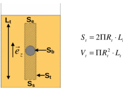
This simplified model allows determining viscosity from the falling ball velocity and the fluid density measurements. In order to be used in the whole range of operating conditions, these experimental densities were previously correlated to an empirical model as the modified Tait equation. We checked that ball velocity is constant and reproducible at a given pressure and temperature. Furthermore, from visual observations, the fluid flow in the tube seems to be similar to a Poiseuille-type flow. The open system considered is the internal volume of the tube with the exclusion of the ball, as it is shown in Fig. 2 (hatched part).
Furthermore we consider the relaxation time (τr), which corresponds to the time for the ball to approach its terminal velocity, such as:
f t f r R µ ρ τ 9 2 =
where Rt is the tube radius (m) and µf is fluid viscosity (Pa.s). For the CB experiments we compared its maximal value (0.3 s) to the minimal time of fall (20 s) - defined by the tube length (0.2 m) divided by the terminal velocity. That is why we can consider a steady flow for the fluid inside the tube.
According to the momentum balance for the fluid (E), the forces exerted on a volume of fluid are the pressure forces (2), gravity forces (3) and viscous friction forces (4), such as:
dS n dV g dS n P dS n v v S f S V f S V r r r r r r ⋅ + + ⋅ − = ⋅
∫∫
ρ ( )∫∫
∫∫∫
ρ∫∫
σ (1) (2) (3) (4) Solenoid Glass tube (a) (b) PistonFor which:
- S is the surface of the considered system composed of four domains, such as:
ball tube s e S S S S S= U U U
- v is the velocity of the fluid (m.s-1) - P is the pressure of the fluid (Pa)
-V
σ is the viscous stress tensor (N.m-2) - V is the internal volume of the system (m3)
- ρfis the density of the fluid (kg.m-3) at given pressure (MPa) and temperature (K), determined from the modified Tait equation [2] such as:
+ + − = 0 0 ) ( ) ) ( ( ln 1 ) , ( ) , ( P T B P T B C P T P T f ρ ρ with 2 2 1 0 ) (T B B T B T B = + ⋅ + ⋅
In which parameters are given as:C= 0.0505; B0= 791.54960; B1= -5.11247; B2= 0.00847; P0=0.1 MPa
Fig. 2 Representation of the system considered for the simplified falling ball model
o Term (1), corresponding to “In-Out” mass balance, is considered to be null because of the following hypothesis:
- vr is null on the tube surface,
- The ball does not roll, thus the fluid velocity vb (m.s
-1
) is identical on the surface Sb, and equal to the velocity of the ball vb:
z b b v e
vr =− ⋅r
-The vertical component of the velocity distribution, vr⋅nr, is identical at the entrance tube (Se) and the exit tube (Ss).
which leads to:
0 ) )( ( ) 1 ( 2 r r r r r r r = ⋅ = ⋅ − − =
∫∫
∫∫
b b b z f b z z S S ρfvbez ve ndS ρ v e e ndSo Term (2), corresponds to the pressure stress balance, such as:
) ( / ) ( / ) ( / ) ( / ) ( / ) ( / ( ) ( ) ) ( ) 2 ( P b f P t f z t f P b f P t f z e s P b f P t f Ss s z Se Pe ezdS P e dS F F P P Se F F gL Se F F r r r r r r r r r r − − = − − − = − − − ⋅ − + ⋅ − =
∫∫
∫∫
ρwhere Lt is the length tube (m) in the hydrostatic pressure term. Ff(/Pt) r and ( ) / P b f F r
are respectively, the pressure forces exerted by the fluid on the tube and on the ball. However, the resultant of ( )
/ P t f F r
is null because of the axisymmetry hypothesis. Moreover, we consider on the entrance surface Se (and respectively on exit surface Ss) that the pressure Pe (and respectively Ps) is uniform, constant and equal to the hydrostatic pressure in the fluid supposed to be motionless outside of the tube. Then:
) ( / ) 2 ( P b f c hydrostati F P r − =
o Term (3), corresponds to the gravity forces balance, such as: ) ( ) 3 ( =− gez Vt−Vb r
ρ where Vb is the ball volume (m3).
o Term (4), corresponds to the viscous forces balance, such as:
) ( / ) ( / ) ( / ) ( / ) 4 ( V b f V t f V b f V t f Ss v Se v ndS ndS F F F F r r r r r r − − = − − ⋅ + ⋅ =
∫∫
σ∫∫
σ where ( ) / V t f F r and ( ) / V b f F rare respectively, the viscous friction forces exerted by the fluid on the tube and on the ball. It is supposed that
]
]
Ss v S v n e n r r ⋅ − = ⋅ σ σ . Se Ss Sb St z
e
r
t t t R L S =2Π ⋅ t t t R L V =Π 2⋅ LtFinally, the momentum balance for the fluid (E) is reduced to: 0 ) ( / ) ( / ) ( / r r r r r = − − − ⋅ V t f V b f P b f z b e F F F gV ρ
According to the fundamental principle of dynamics (E’) applied to a ball which falls at constant velocity without rolling: ) ( / ) ( / 0 V b f P b f z b bgV e F F r r r r − − ⋅
=ρ where ρb is the density of the ball (kg.m-3). Thus, the combination of (E) and (E’) leads to:
z b f b V t f gV e F r r ⋅ − − = ( ) ) ( / ρ ρ
As a first approximation, the fluid flow is a Poiseuille laminar flow (low Reynolds number). Consequently, the flow disturbances near to the ball can be neglected because of the geometric ratio between the ball diameter (2 mm) and the length tube (0.2 m). In this way:
f v L R F t t f b V t f = ⋅ ⋅ 2 ) ( / 2 1 2π ρ r with f=16 Re and Re=2ρfRbvb µf
where f is the friction factor for a laminar flow, Re is the Reynolds number and Rb is the ball radius (m). Thus, after simplifications, it leads to:
µf mod=1
6⋅
(ρb−ρf)⋅g⋅Rb3
Lt⋅vb
This model allows to evaluate the viscosity of the fluid µf mod to initialise CFD calculations of the falling ball for the a more efficient value µf num .
2.3.2 A more efficient falling ball model
Falling ball was modelled using Laminar Navier-Stokes model implemented in commercial software Comsol® Multiphysics 3.4. CFD calculations were carried out in the ball reference (Fig. 3), considering an unsteady and axisymmetric flow with r =0r
ball
v for t=0.
Fig. 3 Representation of the system considered for the CFD falling ball model
The Partial Differential Equations (PDE) system in this 2D geometry is formed by the Laminar Navier-Stokes and the continuity equation for a Newtonian and incompressible fluid:
= ⋅ ∇ + ∇ + −∇ = ⋅ ∇ + ∂ ∂ 0 ) ( ) ( 2 v F v P v v t v f f f r r r r r r r r µ ρ ρ where F r
is the volumetric force exerted on the fluid.
The problem is solved in the accelerating reference system of the ball. In this system F r is such as: ) (v g Fz f b r & r + − = ρ and
in which the acceleration of the ball
v&
b is described according to the fundamental principle of dynamics such as: z b T b f b bv F m g e m r r r & =( ()+ )⋅ / with ) ( / ) ( / ) ( / V b f P b f T b f F F F r r r + = (1) where ( ) / T b f F ris the total volumetric force (viscous and pressure) exerted by the fluid on the ball described by the following integral:
) ) ( ( ( ) ( / n PI v v dS F T S f T b f b
∫∫
⋅ − + ∇ + ∇ = r rr rr rµ with I: identity matrix
Boundary conditions are imposed on the boundary of the considered system as it is shown in Fig. 3.
o Boundary (1), representing the ball surface on which there is a no-slip condition: 0
r r
=
v ,
o Boundary (2) and (6), representing axial symmetry of the tube, 0
= r
F
0 2 4 6 8 10 12 14 0 5 10 15 20 25 P (MPa) µµµµ ( m P a .s )
CFD model Simplified model o Boundary (3), representing the entrance tube. It is an open boundary with a fixed pressure,
o Boundary (5), representing the exit tube. It is an open boundary with a fixed pressure equal to the pressure of the boundary (3) increased by the hydrostatic pressure due to the length of the tube,
o Boundary (4), representing the internal wall surface of the tube. In the reference system of the ball, this wall has a vertical velocity which is calculated at each time step by the integration of the ODE (1). For each CFD calculations, the initial value of the fluid viscosity is estimated by the simplified model value and auto-adjusted with an iteration loop until the ball velocity converges on the measurement value.
2.4. Validation of the experimental set-up
Rheological measurements were achieved with a dynamic rotational rheometer (Haake Rheostress 600, Thermo electron, Germany) with cone-plate geometry (1° angle cone and 60 mm diameter). CB viscosity was measured for temperature ranging from 313.15 to 353.15 K at atmospheric pressure and compared with results obtained with the Falling Ball (FB) viscosimeter and the literature data [1]. CB is a Newtonian fluid and its viscosity decreases exponentially with temperature (Fig. 4).
Fig. 4 Comparison of the measured and literature values for the dynamic viscosity of CB as a function of temperature at atmospheric pressure
Uncertainty in CB viscosity measurements is ±1 % for the FB viscosimeter and the absolute average deviation (AAD) with measurements obtained with the rheometer is 4.5 %.
3. RESULTS AND DISCUSSION
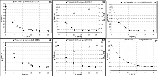
Viscosities were measured for SC-CO2-saturated CB mixture for pressures ranging from 0.1 to 25 MPa at 313.15 and 353.15 K and compared to the results obtained by Venter et al. who performed viscosity measurements using a vibrating quartz viscosimeter (Fig 5(a), 5(b)). The viscosity decreases exponentially with the pressure.
Fig. 5 Comparison of the measurements and literature data for the dynamic viscosity of SC-CO2
-saturated CB at different pressures and at 313.15 K (a, c) and 353.15 K (b, d) and representation of the simplified and the numerical models (e, f)
0 5 10 15 20 25 30 35 40 45 50 0 5 10 15 20 25 P (MPa) µµµµ ( m P a .s )
CFD model Simplified model
0 5 10 15 20 25 30 35 40 45 50 0 5 10 15 20 25 P (MPa) µ µ µ µ (m P a .s ) 0 5 10 15 20 25 30 35 W C O 2 ( % )
Viscosity (mPa.s) wCO2 (%)
0 5 10 15 20 25 30 35 40 45 50 0 5 10 15 20 25 P (MPa) µµµµ ( m P a .s )
This work Venter et al. (2007)
0 2 4 6 8 10 12 14 0 5 10 15 20 25 P (MPa) µµµµ ( m P a .s )
This work Venter et al. (2007)
0 2 4 6 8 10 12 14 0 5 10 15 20 25 P (MPa) µ µµ µ (m P a .s ) 0 5 10 15 20 25 30 35 WC O 2 ( % )
Viscosity (mPa.s) wCO2 (%)
(a) (b) (c) (d) (e) (f) 10 15 20 25 30 35 40 45 303 313 323 333 343 353 T (K) µµµµ ( m P a .s )
The magnitude of decreasing viscosity is about 93 % at 313.15 K and 85 % at 353.15 K. The maximal reduction is reached at approximately 15 MPa as observed by Venter et al. [1]. This tendency is attributed to the CO2 dissolution in the melted media which increases with the pressure (Fig. 5(c), 5(d)). From 15 MPa, the weak decrease of the viscosity is linked to the slow lowering of the CO2 solubility. Furthermore, this behaviour is typical for a binary system in which the components are Newtonian fluids.
Table 1 Experimental results
Fig. 5(e) and 5(f) show a deviation between the predicted and the numerical values of the viscosity which is equivalent to 15.6 % whatever the pressure and the temperature. Thus, taking into account a corrective factor λ=1.185, the simplified model is in very good agreement with the numerical model (AAD=0.12 %). Indeed, CFD calculations show that state of flow is laminar (Re<10) but there are recirculating loops between the ball and the tube. Hence, it means that we cannot consider a Poiseuille-type flow as first approximation in the simplified model. However, the introduction of λ permits to take into account this effect and to simplify easily the determination of the viscosity.
4. CONCLUSIONS
A specific device has been developed for high pressure viscosity measurements of the SC-CO2 -saturated CB mixture. Our results show a good agreement with literature data. This falling ball viscosimeter is a precision tool for the viscosity measurements under high pressure and temperature conditions. Indeed, the relative standard deviation (RSD) ranges between 0.4 and 3.3 %. Thus, there is a good reproducibility between repeated measurements. The precision on measurements is only ±3 %. Our device is now available for further studies about other systems as SC-CO2-polymer and SC-CO2-organic solvent in order to go further in the understanding of the phenomena implied in the crystallization processing.
REFERENCES
[1] M.J. Venter, P. Willems, S. Kareth, E. Weidner, N.J.M. Kuipers, A.B. De Haan, 2007, Phase equilibria and physical properties of CO2 saturated cocoa butter mixtures at elevated pressures, Journal of Supercritical Fluids, 41, 2, p. 195-203
[2] B. Calvignac, E. Rodier, J-J. Letourneau, J. Fages, 2009, Proceedings of the 2nd International congress on Green Process Engineering, Venice, Italy
[3] J-J. Letourneau, S. Vigneau, P. Gonus, J. Fages, 2005, Micronized cocoa butter particles produced by a supercritical process, Chemical Engineering and. Processing, 44, p.201-207
[4] A.R. Bhaskar, S.S.H. Rizvi, C. Bertoli, 1996, Cocoa butter fractionation with supercritical carbon dioxide, Proceedings of the third International Symposium on High Pressure Chemical Engineering, p. 297, Zurich, Switzerland
T (K) P (MPa) v (mm.s-1) ρf (kg.m -3
) µf mod (mPa.s) µf CFD (mPa.s) Confidence interval (mPa.s) Re
0.10 0.39 894.97 38.28 45.38 0.84 0.02 4.23 0.97 902.88 15.28 18.12 0.75 0.10 8.45 2.04 909.89 7.27 8.62 0.25 0.43 10.60 4.15 911.25 3.57 4.20 0.11 1.80 15.90 4.87 920.10 3.03 3.58 0.19 2.50 19.93 5.42 925.12 2.72 3.21 0.22 3.12 25.22 5.54 930.93 2.65 3.14 0.06 3.29 313.15 T (K) P (MPa) v (mm.s-1 ) ρf (kg.m -3
) µf mod (mPa.s) µf CFD (mPa.s) Confidence interval (mPa.s) Re
0.10 1.44 868.18 10.50 12.45 0.35 0.20 5.26 2.76 873.05 5.49 6.51 0.16 0.74 10.09 4.71 876.89 3.21 3.80 0.15 2.17 15.82 7.45 883.15 2.02 2.40 0.03 5.49 19.94 8.70 884.14 1.73 2.05 0.02 7.51 24.10 9.27 887.72 1.62 1.92 0.03 8.57 353.15 P (MPa) T (K) v (mm.s-1
) ρf (kg.m-3) µf mod (mPa.s) µf CFD (mPa.s) Confidence interval (mPa.s) Re
µ (mPa.s) measured by Rheomoter µ (mPa.s) measured by Venter et al. 313.15 0.39 894.97 38.28 44.83 0.84 0.20 43.99 42.05 323.15 0.55 888.28 27.24 32.29 0.88 0.74 30.14 29.21 333.15 0.78 881.59 19.32 22.91 0.83 2.17 22.17 20.93 343.15 1.03 874.90 14.74 17.54 0.72 5.49 16.56 15.59 353.15 1.44 868.18 10.50 12.45 0.35 7.51 13.02 12.14 0.10