Quantifying the overall added value of dynamical
downscaling and the contribution
from different spatial scales
Alejandro Di Luca1, Daniel Argüeso1,2, Jason P. Evans1,2, Ramón de Elía3, and René Laprise4 1Climate Change Research Centre, University of New South Wales, Sydney, New South Wales, Australia,2ARC Centre of
Excellence for Climate System Science, Sydney, New South Wales, Australia,3Consortium Ouranos, Montréal, Québec,
Canada,4Centre ESCER, Département des Sciences de la Terre et de l’Atmosphère, Université du Québec à Montréal,
Montréal, Québec, Canada
Abstract
This study evaluates the added value in the representation of surface climate variables from an ensemble of regional climate model (RCM) simulations by comparing the relative skill of the RCM simulations and their driving data over a wide range of RCM experimental setups and climate statistics. The methodology is specifically designed to compare results across different variables and metrics, and it incorporates a rigorous approach to separate the added value occurring at different spatial scales. Results show that the RCMs’ added value strongly depends on the type of driving data, the climate variable, and the region of interest but depends rather weakly on the choice of the statistical measure, the season, and the RCM physical configuration. Decomposing climate statistics according to different spatial scales shows that improvements are coming from the small scales when considering the representation of spatial patterns, but from the large-scale contribution in the case of absolute values. Our results also show that a large part of the added value can be attained using some simple postprocessing methods.1. Introduction
Nested, limited-area regional climate models (RCMs) began being developed over 20 years ago in order to circumvent the practical impossibility of making operational high-resolution climatic simulations at the global scale. In recent years, the development and use of RCMs have increased, largely due to the strong demand by the climate change impact and adaptation communities that need high-resolution climate projections to perform their studies.
From a science-based perspective, an essential requirement for RCMs to be useful is that they improve some aspect of the simulated climate compared to the global driving data (GDD), i.e., RCMs create some added value (AV) compared to the GDD. As discussed by Hong and Kanamitsu [2014] and Xue et al. [2014], the search for RCM AV has not shown unequivocal gains and the AV has been shown to depend strongly on a variety of factors, including the general setup of the experiment and the specific climate statistics being analyzed. The study of Prömmel and Geyer [2010] may serve to illustrate the strong and complex dependence of the AV on the choice of the climate statistics. Using an AV metric that quantifies the relative performance of the RCM and the GDD to represent monthly time series of 2 m temperature (a combination of correlation and bias), Prömmel and Geyer [2010] showed that the RCM adds little AV and deteriorates some results compared to the GDD in relatively flat subregions surrounding the Alps, particularly during the summer season. They also showed that the RCM tends to slightly outperform the GDD in elevated regions (i.e., with heights above ∼1500 m above mean sea level). Although these results may suggest that RCMs consistently improve 2 m temperature over more complex orography regions, the consideration of only monthly biases shows that the GDD clearly outperforms the RCM in most of these regions throughout the year. As shown by a large num-ber of studies [e.g., Feser, 2006; Winterfeldt and Weisse, 2009; De Sales and Xue, 2011; Kanamitsu and DeHaan, 2011; Dosio et al., 2015], the finding of “mixed results” (i.e., results showing improvements and deteriora-tions depending on the specific climate statistics/experimental setup) constitutes more the standard than the exception in AV studies.
RESEARCH ARTICLE
10.1002/2015JD024009 Key Points:• A rigorous methodology that allows evaluating the overall benefits of high-resolution simulations • The most reliable source of added
value is the better representation of the spatial variability
• Substantial added value can also be attained using simple postprocessing methods
Supporting Information:
• Figure S1 and Text S1
Correspondence to:
A. Di Luca,
Citation:
Di Luca, A., D. Argüeso, J. P. Evans, R. de Elía, and R. Laprise (2016), Quantifying the overall added value of dynamical downscaling and the contribution from different spatial scales, J. Geophys.
Res. Atmos., 121, 1575–1590,
doi:10.1002/2015JD024009.
Received 23 AUG 2015 Accepted 7 JAN 2016
Accepted article online 12 JAN 2016 Published online 26 FEB 2016
©2016. American Geophysical Union. All Rights Reserved.
We know that RCMs provide improvement for specific cases, and we also know of some deteriorations. The question that remains open is which of these two situations is more dominant, that is, whether we can assure that RCMs produce in general—independently of the statistic chosen—a substantial overall improvement over the driving data. The quest of AV in RCMs has some analogies with studies trying to establish the overall skill of the different generations of the Coupled Model Intercomparison Project (CMIP) models [Reichler and Kim, 2008; Flato et al., 2013; Watterson et al., 2014]. These studies are generally used to justify the develop-ment of higher-resolution models tending to include more complex processes even when the improvedevelop-ments between, for example, the phase 5 of CMIP (CMIP5) and the earlier phase 3 (CMIP3) are found to be quite limited and more a property of the ensemble than of individual models. It is in the light of the general diffi-culties in finding improvements between model generations that the quest of AV in RCMs should receive a fairer assessment.
This study addresses the question of the general improvement of RCMs by performing an “overall” evaluation of the AV generated by RCMs using a range of experimental setups (driving data sets, resolutions, etc.) and surface climate statistics (various variables, seasons, regions, etc.). The evaluation is performed using an innovative methodology that includes
1. A systematic sampling of factors that influence the AV including various experimental setups, several variables, and a range of statistical measures, seasons, and regions.
2. Two AV metrics that characterize the relative performance of the RCM and the GDD based on the represen-tation of absolute values (mean square error (mse) AV metric) and spatial patterns (spatial correlation AV metric). In addition, both AV metrics are normalized allowing results from different climate statistics to be compared directly.
3. A spatial-scale decomposition method that allows separation of the AV according to the contribution from large (i.e., GCM permitted) and small (i.e., RCM permitted) spatial scales.
The analysis uses data from the largest RCM ensemble available over southeast Australia. Although this ensemble allows for a good sampling of some key factors affecting the AV of RCMs such as a variety of parameterizations, two resolutions (i.e., 10 and 50 km grid spacing), and a range of distinct climates, it is restricted to three GDD and three RCMs that are based on the Weather Research and Forecasting System. Maybe more importantly, the analysis is restricted to a few surface variables (namely, minimum and maximum temperature, and precipitation) available at daily frequency due to the lack of high-resolution observations of other surface variables.
The paper is structured as follows. Section 2 presents a brief description of the data used, and section 3 describes the spatial-scale decomposition method together with the metrics used to quantify the AV. Section 4 presents results for the overall AV and the contribution of the different spatial scales to the improvements/deteriorations. Lastly, discussion and concluding remarks are given in section 5.
2. Data
Daily gridded data from the Australian Water Availability Project (AWAP) [Jones et al., 2009] are used in this study as the reference data set. AWAP is a product developed by the Bureau of Meteorology of Australia con-sisting of daily gridded data sets of in situ measurements of minimum and maximum 2 m temperatures, and precipitation on 0.05∘ by 0.05∘ grids.
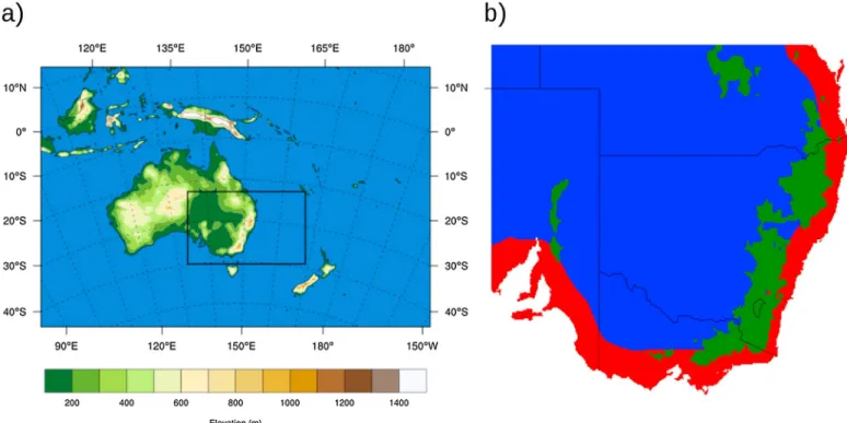
The RCM ensemble used here was performed in the context of the NARCliM (NSW/ACT Regional Climate Modelling) project. It consists of a total of 18 RCM simulations performed using three different RCM versions, two different spatial resolutions, and three different sources of GDD. Simulations were carried out using a double-nesting approach where the GDD are used to drive the RCM at 50 km grid spacing over a domain that covers the Coordinated Regional Climate Downscaling Experiment (CORDEX)-Austral Asia region (RCM50, Figure 1), and then the RCM50 is used to drive the same RCM with a horizontal grid spacing of 10 km over a domain that includes southeast Australia (RCM10, black rectangle in Figure 1). The three different RCM ver-sions were constructed using version 3.3 of the Weather Research and Forecasting (WRF) [Skamarock, 2004] RCM by combining different surface/planetary boundary layer, cumulus, and atmospheric radiation schemes, and all three versions share the dynamical core, the Noah land surface scheme, and the microphysics scheme. These three WRF versions were selected from a 36-member multiphysics ensemble based on their model skill and independence in a two-step selection process [Evans et al., 2012, 2014]. First, individual members of the
Figure 1. (a) The 50 km RCM simulations domain (CORDEX-Austral Asia domain) and the 10 km RCM domain (black rectangle) and (b) the three regions of
analysis: coastal (red), complex topography (green), and flat (blue) regions.
full multiphysics ensemble are evaluated over southeast Australia in order to remove from the ensemble those models that are not able to adequately simulate the climate. Second, from the subensemble obtained in the former step, a subset is chosen such that each selected member is as independent as possible from the others. The independence was measured using a recent method developed by Bishop and Abramowitz [2013] that uses the covariance in model errors as the basis for a definition of model independence. Indeed, selected WRF versions correspond to three of the most independent/best performing models of the 36-member ensemble. Although, as mentioned above, the selection process explicitly addresses the independence between mem-bers of the ensemble, it is still unclear how independent these WRF versions are compared with what would be obtained using three “totally independent” RCMs (e.g., three RCMs developed independently by different modeling groups). Various studies [e.g., Argüeso et al., 2011; Jerez and Montavez, 2013; Di Luca et al., 2014] have shown that the spread associated with multiphysics ensembles can be as large as the spread obtained using multimodel ensembles depending on the variable being considered with precipitation showing relatively more dependence on the physics than more dynamical variables such as evaporation and possibly tempera-ture. That is, although we had explicitly considered the independence issue in the selection of the RCMs, we cannot rule out that some common behaviors across the WRF versions can arise. For further details on the ensemble and the NARCliM experiment design, the reader is referred to Evans et al. [2014].
Surface and lateral boundary conditions used to drive the 50 km RCMs are provided by the NCEP-NCAR reanalysis 1 (NNRP) [Kalnay et al., 1996] and two simulations performed using the fifth version of the European Centre/Hamburg (ECHAM) GCM (ECHAM5) [Roeckner et al., 2003] and the version 3.1 of the Canadian Centre for Climate Modelling and Analysis (CCCMA) GCM (CCCMA3.1) [Kim et al., 2002]. The approximate horizon-tal grid spacing of the NNRP, ECHAM5, and CCCMA3.1 products is 300 (T62), 300 (T63), and 450 (T42) km, respectively.
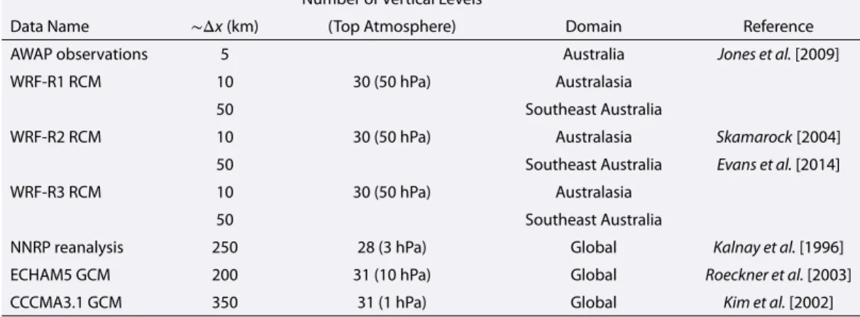
An overview of the data is presented in Table 1. It should be noted that resolution differences between RCM simulations and GDD are not only related to the horizontal but also with the vertical resolution. All simulations and reanalysis have a similar number of vertical levels (between 28 and 31), but the distribution of the vertical levels varies across the various data sets.
Table 1. Overview of the Observations, and Regional and Global Climate Simulations Used in the Studya
Number of Vertical Levels
Data Name ∼Δx(km) (Top Atmosphere) Domain Reference AWAP observations 5 Australia Jones et al. [2009] WRF-R1 RCM 10 30 (50 hPa) Australasia
50 Southeast Australia
WRF-R2 RCM 10 30 (50 hPa) Australasia Skamarock [2004] 50 Southeast Australia Evans et al. [2014] WRF-R3 RCM 10 30 (50 hPa) Australasia
50 Southeast Australia
NNRP reanalysis 250 28 (3 hPa) Global Kalnay et al. [1996] ECHAM5 GCM 200 31 (10 hPa) Global Roeckner et al. [2003] CCCMA3.1 GCM 350 31 (1 hPa) Global Kim et al. [2002]
aData name, horizontal grid spacing (Δx; in kilometers), number of vertical levels and pressure of the highest level,
domain, and reference for each data set. Differences between the three WRF configurations are given by the different choice of the radiation, planetary boundary/surface layer, and cumulus parameterizations schemes.
3. Methods
The methodological approach followed here includes the calculation of various climate statistics, the use of a spatial-scale decomposition method, the interpolation of the decomposed terms onto a common grid mesh, and the computation of two different metrics quantifying the resulting AV. These steps are described in some detail in the following sections.
3.1. Climate Statistics and Spatial-Scale Decomposition
The aim of this section is to present an approach allowing comparison of GDD/RCM data with observations by explicitly evaluating their performance at different spatial scales. Following Di Luca et al. [2013a], a climate statistic X (e.g., seasonal mean precipitation) calculated from time-varying 10 km grid-spacing observations (o(x, y, t)) can be separated according to different spatial scales as follows:
XOBS= XOBS300+ X 50′ OBS+ X 10′ OBS. (1) The term X300
OBSrepresents the climate statistic X calculated using the time-varying observations after they
were upscaled over a mesh with a 300 km grid spacing. The upscaling is performed by simply aggregating the high-resolution values within the lower resolution grid boxes. The superindex 300 in equation (1) is taken as a nominal value to designate the part of the climate statistics that can be represented by the driving data, although the actual grid spacing depends on the particular GDD used and it may be somewhat different from 300 km (e.g., about 450 km for the CCCMA3.1 GCM).
The term X50′
OBSis given by the difference between the climate statistic X calculated using observations that
were upscaled over the 300 km and the 50 km grid meshes (i.e., X50′
OBS= X
300
OBS− X
50
OBS). Defined in this way, the
term X50′
OBScontains the extra information provided by the 50 km data compared to the 300 km data. Similarly,
the term X10′
OBSincludes the extra information provided by the very high resolution climate statistic (i.e., 10 km
grid spacing) compared with the 50 km climate statistic (i.e., X10′
OBS = X
50
OBS− X
10
OBS). Clearly, whenever X 50′
OBSor
X10′
OBSis very small compared with X 300
OBSit means that the large-scale part dominates the field XOBSwith little
impact of fine spatial-scale structures.
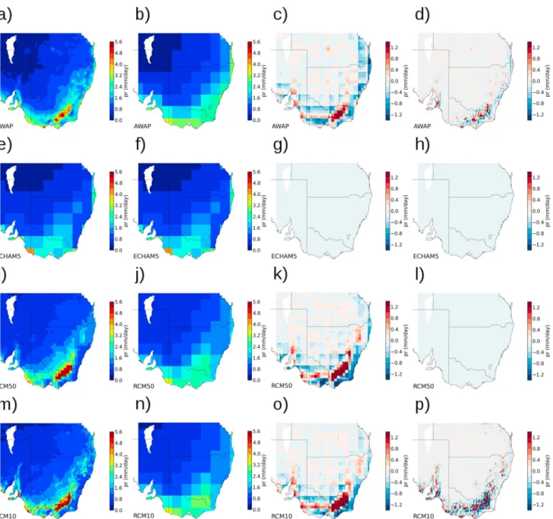
To illustrate the spatial-scale decomposition, Figures 2a–2d show the mean summer precipitation for the high-resolution 10 km AWAP field (XOBS; Figure 2a) together with its large-scale term (XOBS300; Figure 2b), its
small-scale term (X50′
OBS; Figure 2c), and its very small scale term (X 10′
OBS; Figure 2d) as described in equation (1).
The mean precipitation shows substantial fine-scale details particularly in the southeast part of the domain and, more generally, near the coast where surface forcings are more important. The large-scale term (Figure 2b) shows a general increase of the precipitation as we moved toward the coast from the center of Australia. As expected, the large-scale term is not able to represent the variability of precipitation around the mountains particularly in the southeast part of the domain. However, the fine-scale details in the precipitation
Figure 2. Summer mean precipitation for (a–d) the AWAP observations, (e–h) the ECHAM5 GCM, and (i–l) the 50 km and (m–p) the 10 km RCM (version R1).
Different columns show results for the various terms of the decomposition presented in equations (1)–(4): total (X, first column), large scale (X300, second column),
small scale (X50′
, third column) and very small scale (X10′
, fourth column).
field appear in the small-scale (Figure 2c) and very small scale (Figure 2d) terms. In some regions, the contribu-tion from fine scales can be as large as the large-scale term (e.g., near the Snowy Mountains in the southeast part of the domain), although in general it is much smaller.
Applying the spatial decomposition to the GDD and the 50 and 10 km RCM data, we obtain
XGDD= XGDD300, (2)
XRCM50= XRCM50300 + X 50′
and XRCM10= XRCM10300 + X 50′ RCM10+ X 10′ RCM10, (4) with X50 GDD = X 10 GDD = X 10
RCM50 = 0. Figure 2 shows the mean summer precipitation and their
correspond-ing decomposed fields for the ECHAM5 GCM (Figures 2e–2h), the RCM50 (Figures 2i–2l), and the RCM10 (Figures 2m–2p).
3.2. High-Resolution Grid Interpolation
In order to directly compare results from data sets available over different grid meshes, we need to make two choices (see Prein et al. [2015] for a discussion). The first is the choice of a common grid where comparisons will be performed. Hong and Kanamitsu [2014] argued that “all of the comparisons need to be made on the coars-est resolution among the observations, the global model, and the regional model... [and]... the interpolation needs to be performed by taking the scale into consideration.” In the context of the spatial-scale decompo-sition method applied here, the use of the highest-resolution grid mesh (10 km grid mesh) as the common grid is the natural choice because the other alternatives, namely, the 50 km grid or the GDD grid meshes, are explicitly considered as part of the spatial decomposition. This implies that our analysis simultaneously assesses the AV over those spatial scales that are common to both the RCMs and the GDD (denoted here as large scales) but also the AV arising from spatial scales that are finer than the GDD grid (denoted here as small and very small scales).
The second important choice is related to the method used to interpolate from the coarser to the finer grid. In this study, we focus on results obtained using a “nearest-neighbor” method to interpolate all fields to the highest resolution grid mesh (this method would lead to similar results as the “conservative resampling procedure” used by Prein et al. [2015]). The use of this method ensures that the new high-resolution interpo-lated field conserves the spatial variability and the areal-averaged values compared with the original field. A disadvantage is that contrary to results that would be obtained using bilinear or cubic spline interpolation methods, the nearest-neighbor method somewhat penalizes lower resolution data sets (e.g., GCM or RCM50 results) which will appear as a set of large pixels with uniform values.
To take into account the uncertainty in the AV arising from the choice of the method used to interpolate low-resolution fields into the high-resolution grid, we have performed two additional sets of calculations using alternative methods. The first one simply uses a bilinear interpolation method instead of the near-est neighbor to interpolate from a coarse to a finer grid. The second is somewhat more sophisticated, and, on top of a bilinear interpolation, it includes a correction to account for the dependence of 2 m temper-ature on elevation (topography correction). More specifically, the topography correction is performed by adding the difference between the high-resolution and low-resolution topography fields multiplied by the middle-latitude standard atmosphere lapse rate (Γ = −6.5 K/km). The elevation correction is applied to minimum and maximum temperature fields from the 50 km RCM simulations and the GDD data. A similar correction was applied in other studies [Prömmel and Geyer, 2010; Di Luca et al., 2013b; Prein et al., 2013]. Figure S1 in the supporting information illustrates differences across the three interpolation methods for the minimum temperature field. Results from the bilinear plus topography correction method show a much higher level of fine-scale detail than results obtained using only bilinear interpolation and mostly compared with the nearest-neighbor method. Clearly, the use of bilinear interpolation constitutes a better approxima-tion of the likely variaapproxima-tion of the temperature field inside original grid boxes thus favoring the low-resoluapproxima-tion models in the comparison.
3.3. AV Metrics
Once we have calculated the climate statistics for each data set (AWAP, GDD, and RCM simulations) and for the various spatial scales, the next step is to estimate the AV. As suggested by Di Luca et al. [2015], the AV of an RCM over the GDD can be quantified by comparing the relative skill of the GDD and RCM to represent the observed statistic:
AVd= d(XGDD, XOBS) − d(XRCM, XOBS), (5)
where d represents some distance metric between a given data set and the observations. Defined in this way, an RCM generates some AV if AVdis larger than 0, i.e., if the RCM constitutes a better approximation of the observed field compared to the GDD. In equation (5), subindex RCM denotes results derived from either the 10 km grid spacing RCM (RCM10) or the 50 km grid spacing model (RCM50).
Following Di Luca et al. [2013a], a simple AV metric can be obtained by using the mean square error (mse) as distance metric between a simulated data set and observations:
AVmse= (XGDD− XOBS)2− (X
RCM− XOBS)2
= mseGDD− mseRCM, (6)
with ()2denoting the average of the square differences between observed and simulated climate statistics X
over all grid points in the region of interest. That is, the mse AV metric evaluates the relative performance of the GDD and the RCM across the distinct regions (i.e., flat, land-sea contrast, and complex topography regions) without the explicit consideration of results at specific grid points.
Replacing equations (1), (2), and (4) in equation (6) and rearranging, we obtain an expression for the AV of the 10 km grid spacing RCMs:
AVmse,RCM10= AV300mse,RCM10+ AV50mse,RCM10+ AV10mse,RCM10+ AVmse,RCM10cov10, (7)
where expressions for the various terms in equation (7) are presented in detail in the supporting informa-tion. Here we note that the total AV of the 10 km RCM (AVmse,RCM10) can be decomposed into a large-scale
(AV300
mse,RCM10), a small-scale (AV
50
mse,RCM10), a very small scale (AV
10
mse,RCM10), and a covariance (AVmse,RCM10cov10)
component. The large-scale term represents the difference between the mse of the GDD field and the large-scale part of the RCM field. The small-scale term (AV50
mse,RCM10) quantifies the difference between the mse
and the total variance of the small-scale part of the RCM field. A similar interpretation follows for the very small scale term (AV10
mse,RCM10). For a more detailed discussion about the meaning of every term, see Di Luca
et al. [2013a].
A second AV metric can be obtained using the error in the spatial correlation calculated between climate statis-tics obtained from the observed and the simulated (i.e., GDD and RCM) variables, that is, d = 1 − corr(X, XOBS).
In this case we obtain the following expression for the AV metric:
AVcorr= (1 − corr(XGDD, XOBS)) − (1 − corr(XRCM, XOBS))
= corr(XRCM, XOBS) − corr(XGDD, XOBS). (8)
Replacing equations (1), (2), and (4) in equation (8), we obtain an expression of the correlation AV metric that depends on the contribution of the various spatial-scale terms:
AVcorr,RCM10= AV300corr+ AV50corr+ AV10corr. (9)
Again, the term AV300
corrquantifies the AV in the correlation coefficient that arises from a better representation
of the large-scale part of the field, while the terms given by AV50 corrand AV
10
corrcorrespond to the AV arising from
the representation of the fine-scale spatial variability that is absent in the 300 km and the 50 km grid mesh, respectively. More detailed expressions for each term are presented in the supporting information.
In order to compare AV results obtained from using different climate statistics (i.e., different variables, regions, seasons, etc.), we proceed to normalize both AV metrics by the sum of the RCM and GDD errors:
̂ AVd=
d(XGDD, XOBS) − d(XRCM, XOBS) d(XGDD, XOBS) + d(XRCM, XOBS)
. (10)
Defined in this way, ̂AVmseand ̂AVcorrquantify the total AV relative to the error in the GDD and the RCM. Both
quantities vary between −1 and 1 with larger positive values suggesting smaller RCM errors than the GCM errors and thus a substantial AV from the RCM.
3.4. Factors Influencing the AV
As discussed by Di Luca et al. [2015], the factors influencing the AV can be separated into those related to choices in the experimental setup and those related to choices in the climate statistic (see Table 2). Among the experimental setup factors, here we included the choice of the horizontal resolution (two options) and RCM’s version (four: three different versions and the ensemble mean of the RCMs) and the choice of the GDD (three). Among the factors related to the climate statistic we have the choice of the season (four), region (three), vari-able (three), and statistical measure (three). Tvari-able 2 gives more details on the specific values of the several factors considered in the analysis.
Table 2. Name, Source, Number, and Particular Values of the Various Factors Influencing the AV That Are Considered in
the Analysisa
Factor Source Number Options Season CS 4 DJF, MAM, JJA, and SON
Region CS 3 coastal (coast), complex topography (topo), and flat
dx(RCM) ES 2 10 and 50 km grid spacing simulations RCM ES 4 R1, R2, and R3, and ensemble mean (EM) GDD ES 3 NNRP, CCCMA3.1, and ECHAM5 Variable CS 3 2 m minimum temperature (tmin), 2 m maximum
temperature (tmax), and precipitation (pr) Measure CS 3 mean, standard deviation (stddev), and 99th percentile (q99)
aFactors related to the experimental setup are denoted by ES and those associated with the choice of the climate
statistic by CS. Abbreviations as used in the legends of the figures are also included. DJF, December-January-February; MAM, March-April-May; JJA, June-July-August; and SON, September-October-November.
Calculations are performed separately for three distinct regions that are characterized by complex topography (grid points with an elevation higher than 500 m), land-sea contrasts (grid points that are within 150 km from the coast), or a relatively smooth terrain far from the coast (see Figure 1b). Grid points that are characterized by both complex topography and land-sea contrasts are considered to belong to the complex topography region.
All statistics are calculated using daily 20 year time series from the period between 1990 and 2009, and the analysis is limited to those variables available in the AWAP data set, thus, 2 m minimum and maximum tem-perature, and precipitation. Note that the combination of all the factors considered in this analysis (see third column in Table 2) leads to a total of 2592 AV estimates for each AV metric.
4. Results
4.1. Overall Added Value
Figures 3a and 3b show the total AV averaged over individual values of the different factors for the ̂AVmse
(Figure 3a; see equation (6)) and the ̂AVcorr(Figure 3b; see equation (8)) metrics. For example, the season
column shows four values, one for each season, that were obtained by averaging the ̂AV matrix across all other factors while leaving constant the season specified.
Results for the mse AV metric ̂AVmse(Figure 3a) show that the overall AV is positive and about 30% of the sum of mean square errors in the RCM and the GDD. The largest variations of the mean AV are related to the choice of the GDD and the choice of the variable. In particular, the AV of RCMs is smallest when considering simulations driven by the NNRP reanalysis and largest when simulations are driven by the CCCMA3.1 data. This behavior is partially explained by the smaller mses in the NNRP data than in the CCCMA3.1 data. A lower mse in the NNRP is expected since reanalyses are built using observations. Regarding the choice of the variable, the largest AV arises when considering both minimum and maximum 2 m temperatures while the precipitation variable shows that on average the AV is slightly negative (∼-0.05). To a lesser extent, the choice of the region seems to be important with the largest improvements appearing in coastal or complex terrain regions. Seasonal differences show that the AV is much larger in winter (JJA) and autumn (SON) than in the summer (DJF) season. For the correlation AV metric ̂AVcorr(Figure 3b), we again found that overall, the RCMs improve on their
corre-sponding GDD with an average increase of about 30% of the sum of correlation deficits in the RCM and the GDD. The amelioration in the representation of spatial patterns is rather consistent across the various factors. Regions with complex topography show larger improvements than flat and coastal regions. Also, the temper-ature variables (tmin and tmax) show more AV than precipitation, although differences between variables are not as large as for the mse AV metric. Ameliorations arising for the precipitation variable suggest that RCMs produce a better spatial distribution of precipitation even though they do not improve the absolute values in our study.
The choice of the source of GDD again plays a key role with the largest gains arising when comparing with the CCCMA3.1 GCM simulation. It is worth noting that contrary to the AV mse metric, substantial AV for the correlation AV metric is associated with the NNRP as a driver and this AV is even larger than that associated
Figure 3. (a, b) The total AV averaged over specific values of the various factors considered in the analysis and (c, d) the
percentage of times that there is some AV (i.e., AV is positive) for specific values. Figures 3a and 3c show results for the mse AV metric and Figures 3b and 3d results for the correlation AV metric. Averaged AV values are normalized as explained in section 3.3. The RCM adds value over the GDD whenever values are higher than 0 and 50% for the mse and correlation AV metrics, respectively. To improve readability, specific values of a given factor are slightly offset in the horizontal.
with the ECHAM5. The last results suggest that the main factor determining the AV in the spatial correlation metric is related to the jump in the horizontal resolution between the RCM simulation and the GDD that is largest for the CCCMA3.1 GCM and smallest for the ECHAM5 GCM.
Regardless of the AV metric considered, differences between the AV obtained using different versions of the WRF model are relatively small, although version R3 systematically shows less AV than any other version including the ensemble mean WRF obtained by averaging the climate statistics across the three WRF versions.
An alternative way of quantifying the overall AV is by calculating the number of climate statistics/experimental setups, for any given factor, for which the ̂AV matrix has a positive sign (i.e., “sign AV” quantity). Such a measure has two main advantages. First, it is not biased toward those parameters showing very large values of AV (e.g., the complex topography region), and second, it allows a fair comparison between the mse and the correlation AV metrics. That is, instead of calculating the average AV across all experimental setups and climate statistics for every single factor, we calculate the proportion of times that the sign of the AV metric is positive. In this way, whenever the percentage of positive AV values is higher than 50% it means that the RCM improves more often than it deteriorates upon the GDD.
Table 3. Estimated AV Values for Various Specific Key Factorsa
DJF JJA
AV metric Region Variable mean q99 mean q99
mse coast pr −0.64 −0.32 0.07 0.40 tmax 0.92 0.73 0.90 0.83 flat pr −0.79 −0.71 −0.24 0.30 tmax 0.96 0.86 0.90 0.90 corr coast pr −0.22 −0.09 0.11 0.39 tmax 0.28 0.22 0.17 0.09 flat pr 0.28 0.31 0.13 0.33 tmax 0.35 −0.01 0.39 0.32
aAV values correspond to results obtained using the 10 km grid spacing R1 WRF version driven by the ECHAM5 GCM.
For the mse metric (Figure 3c), results show that about 72% of the cases under study display some form of AV. The sensitivity of the sign AV quantity to the various factors is in agreement with results obtained using the “averaged AV” metric with a few small differences. For example, although the mean AV for the precipitation variable was negative, slightly more than 50% of the total cases show positive AV values. Another interesting difference is that between JJA and SON for the mse AV metric. While the mean AV shows nearly the same values for both JJA and SON seasons, the sign AV metric shows substantially higher values in the austral winter (80%) than in the spring (72%).
For the correlation AV metric (Figure 3d), results show that about 85% of the cases under study display some form of AV. This result suggests that overall, the chances of improving the representation of the spatial pattern are higher than those of diminishing mean square errors.
Results presented in this section pull together contributions across all factors being considered without any detailed information of individual contributions to the overall AV. As a consequence, a direct comparison of our results with other studies may be difficult to perform. Table 3 includes specific AV values for some of the key factors considered in the analysis: two seasons (JJA and DJF), two variables (precipitation and maximum temperature), two statistical measures (mean and 99th percentile), and two regions (flat and coastal) for only one WRF version (R1), one resolution (10 km), and one global driving data (ECHAM5 GCM). Moreover, Figure 3 informs us about the overall AV for all cases, but it is mute with respect to the contribution of each spatial scale. Section 4.3 concentrates on this issue.
4.2. The 10 km Versus 50 km RCM Added Value
For both the mse and the correlation AV metrics (Figure 3), the 10 km RCM adds more value than the 50 km ver-sion, suggesting that overall the improvement becomes larger as the horizontal resolution increases. Clearly, the increase in resolution from 10 to 50 km grid mesh has a larger impact on the correlation AV metric than the mse AV metric. Specifically, it is seen that differences between the 10 km and 50 km simulations explained 28% of the total 10 km RCM AV in the case of the correlation AV metric and only about 17% in the case of the mse AV metric.
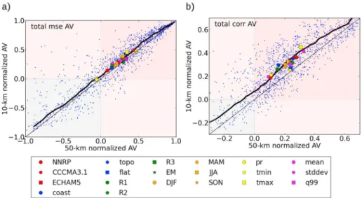
To gain further insight into the comparison between the two resolution RCM simulations, Figure 4 shows the 10 km total AV values as a function of the 50 km values for the mse (Figure 4a) and the correlation (Figure 4b) AV metrics. For both AV metrics, there is a strong correlation between the AV obtained using both resolution RCM simulations. A moving average across different bins (thick black line) between the 10 and 50 km AV indicates that 10 km simulations systematically show higher AV regardless of the absolute values of the AV (i.e., thick black line is displaced to the left of the one-to-one line). As mentioned before, the increased resolution from 50 to 10 km has a larger impact when considering the correlation AV metric compared to the mse AV metric. 4.3. Spatially Decomposed Added Value
Figure 5a shows the total AV (top row) for the mse AV metric using the 10 km simulations together with the contribution from the different spatial scales (other rows) as a function of the various factors (in columns). For any given factor and spatial scale, the mean AV for specific values of the factor is shown. For example, the four squares in the top left corner show the total AV averaged across results from simulations using the CCCMA3.1,
Figure 4. Scatterplot between the mean AV in the RCM10 and the RCM50 for (a) the mse AV metric and (b) the
correlation AV metric. Mean values across individual factors are shown using different colors and symbols. The black thick line shows a moving average across different bins. The grey region designates the area where both RCM
resolutions (i.e., RCM10 and RCM50) deteriorate upon the GDD. Pink regions designate those areas where either both or one of the RCMs improve upon the GDD.
the NNRP, and the ECHAM5 GDD, respectively. It should be noted that the sum of the AV values across the different decomposition terms is equal to the total AV (see equations (7) and (10)).
Results for the mse metric using 10 km simulation (Figure 5a) show that the total AV is mostly determined by the contribution of the large-scale term (AV300
mse,RCM10) with occasionally a nonnegligible influence of the
covariance term (AVmse,RCM10cov10). The 50 km AV term (AV50
mse,RCM10) is generally negative although quite small
compared with the large-scale part. The 10 km AV term (AV10
mse,RCM10) is generally negative, although very
close to zero, suggesting that on average this term tends to slightly deteriorate the representation of the total statistic.
It is interesting to note that when considering the total AV derived from RCM simulations performed using the NNRP as GDD, a large proportion of AV comes from the 50 km AV term showing that the use of “near-perfect boundary conditions” strongly limits the generation of AV at large scales.
Results for the correlation AV metric using 10 km simulations (Figure 5b) show that the total AV is largely dominated by the contribution of the small-scale and very small scale AV terms (i.e., 10 and 50 km spatial scales) with generally negative but small values for the large-scale term. It is worth noting a few exceptions to the last result. Over flat regions and for the maximum temperature, improvements in the spatial pattern are determined by the large-scale term with small contributions from the small-scale terms. As might be expected, the contribution from the 10 km term is particularly important in the region with complex topography and for the precipitation variable.
Results obtained using the 50 km simulations (Figures 5c and 5d) are very similar to those using the 10 km simulations. Again, the spatial-scale decomposition of the mse AV metric shows that improvements come from the large-scale term while the correlation AV metric is dominated by the 50 km spatial-scale term. 4.4. Added Value Using Other Interpolation Methods
As discussed in section 3.2, the choice of the nearest-neighbor method to interpolate low-resolution fields into the high-resolution grid mesh might be somewhat “unfair” for the low-resolution fields. Figure 6 shows the overall AV for three different interpolation methods: nearest neighbor, bilinear (denoted as “linear”), and bilinear including a simple topographic correction (“linear + topo”; see description in section 3.2). Results are shown independently for the three different variables (rows: tmin, tmax, and pr) and two regions (columns: flat and complex topography). Each plot shows the mse (full lines) and the correlation (dashed lines) AV metrics together with the 10 and 50 km RCMs (red and blue colors, respectively).
Figure 6 shows that with the exception of the mse AV metric for precipitation, the overall AV is positive irre-spective of the region, variable, AV metric, RCM resolution, and interpolation method considered. It is clear,
Figure 5. Total AV terms and the contribution from different spatial scales as a function of the various factors of interest
for (a and c) the mse and (b and d) the correlation AV metrics. Results obtained using the 10 and 50 km simulations are shown in Figures 5a and 5b and Figures 5c and 5d, respectively. Note that a square is assigned to each factor and AV scale term and that each quadrant of the square gives the averaged AV for specific values of each factor. Hence, the lower right quadrant of the square located in the “region” column and the “300” AV term row represents the averaged AV over the “flat region” for the large-scale term.
however, that the RCM’s AV diminishes as we account for the likely spatial variation in the lower resolution fields (GDD and 50 km RCM fields) using the bilinear interpolation (“linear” column). For temperature vari-ables, decreases in the AV introduced by the bilinear interpolation vary between 10 and 40% of the original AV value depending on the variable and the metric considered. For the precipitation variable, the bilinear interpolation does not play a substantial role and the AV shows only a slight decrease of about 10% for the correlation metric.
After the topographic correction is applied to lower resolution temperature fields (linear + topo column), the AV decreases even more than when only considering the bilinear interpolation. As expected, the AV decreases more over regions with more complex topography compared with flat regions. For example, for the minimum temperature in complex topography regions, the AV decreases by 50 and 80% for the mse and the correlation AV metric, respectively. In general, the AV using the spatial correlation metric shows larger variations than the mse metric.
It is also interesting to consider changes in the AV between the two RCM resolution simulations after the simple postprocessing methods were applied to the 50 km statistics. While using the nearest-neighbor inter-polation the 10 km resolution produced 17 and 28% more AV than the 50 km resolution simulations, these values drop to 13 and 18% for the mse and correlation AV metrics, respectively. This suggests that a substan-tial part of the improvement obtained when increasing the resolution from 10 to 50 km can be attained using simple postprocessing of the 50 km resolution RCM.
Figure 6. Overall AV for (a, b) minimum temperature, (c, d) maximum temperature, and (e, f ) precipitation for flat
(Figures 6a, 6c, and 6e) and topo (Figures 6b, 6d, and 6f ) regions calculated using three different interpolation methods as described in section 3.2. Interpolations performed using a nearest neighbor, a bilinear, and a bilinear including the topographic and land-sea mask corrections are denoted as “nearest,” “linear,” and “linear + topo,” respectively. Red lines show results for the 10 km RCM for the mse (full line) and the correlation (dashed line) AV metrics. Blue lines show results for the 50 km RCM for the mse (full line) and the correlation (dashed line) AV metrics.
5. Discussion and Conclusions
The purpose of this study was to establish whether one of the RCM ensembles available to the RCM commu-nity, the NARCLIM data set centered over Australia, showed overall signs of AV (added value) with respect to the driving data and at which spatial scale this AV occurred.
We have evaluated the overall AV of an 18-member ensemble of RCM simulations and its partial dependence on several factors related to the experimental design and to the climate statistics of interest based on two dif-ferent metrics. A first metric, denoted as mse AV metric, quantifies the relative performance of the RCM and its driving data to represent local values of climate statistics from a mean square root perspective. The sec-ond metric, denoted as correlation AV metric, quantifies the improvements/deteriorations produced by the RCM in representing the spatial patterns of the climate statistics. Both AV metrics were further decomposed into the contribution from different spatial scales, including the finest spatial scales permitted by the RCMs and the driving data. The evaluation was performed using the 0.05∘ by 0.05∘ AWAP gridded data set of daily
observed precipitation and minimum and maximum temperature. Although the AWAP data set appears to be reasonably consistent with station values [e.g., King et al., 2013], climatological errors resulting from low station density are expected to be important toward central Australia (where station density is very low) and over complex topography (where precipitation is highly spatially inhomogeneous). AWAP errors are expected to have a larger impact particularly when looking at very fine scale features.
Our results indicate that for both AV metrics, the performance of RCMs is superior compared to the corre-sponding driving data. We found overall improvements of 0.27 for both the normalized mse and correlation AV metrics (i.e., almost 30% improvement). We have also found that in 72% and 85% of the cases the RCM adds value to the driving data for the mse and the correlation AV metrics, respectively. Clearly, although we have tried to sample the range of factors affecting the amount of AV as much as possible, our results are limited in at least two regards. First, the specific ensemble considered is restricted to three GDD and three WRF versions that are not completely independent (e.g., WRF versions share the dynamical core and land surface scheme). Second, the analysis is limited to three surface variables (i.e., minimum and maximum temperature, and pre-cipitation) due to the lack of high-resolution observations of other quantities (e.g., wind field, humidity, and evaporation) over southeast Australia.
In general, our results regarding the dependence of the AV on the various factors considered fall in line with earlier research. It should be kept in mind, however, that a direct comparison with other studies is precluded because our metrics “merge” results from a variety of statistics, variables, regions and seasons, instead of rep-resenting single quantities (e.g., long-term mean precipitation) as in most studies. Still, our findings indicate that in agreement with many other studies [e.g., Feser, 2006; Winterfeldt and Weisse, 2009; Prömmel and Geyer, 2010; Feser et al., 2011; Di Luca et al., 2013b; Prein et al., 2015], the largest AV appears in regions characterized by either complex topography or by land-sea contrasts. We also found that the AV is largest when consid-ering more extreme statistical quantities (i.e., 99th percentile) for the mse AV metric and when considconsid-ering long-term seasonal mean values for the spatial correlation metric. In particular, regardless of the AV metric considered, the temporal standard deviation shows the smallest AV, perhaps due to its relatively low spatial variability over complex topography regions.
Regarding the seasonal dependence, for the mse AV metric we found that the largest AV values appear in aus-tral winter and the lowest in summer. Further inspection of this result indicates that these seasonal differences are dominated by the seasonal differences in the precipitation variable with temperature variables showing relatively small seasonal differences. The reason why the precipitation AV is smaller in summer than in winter appears to be related to a generally poorer ability of the RCM ensemble to simulate summer precipitation, particularly over the north of the domain where RCMs produce quite large overestimations.
Decomposing the AV according to the contribution of different spatial scales gives more insight into the sources of AV and allows identification of a major difference between the AV in the mse and the correlation metrics:
1. The AV related to the local values of the climate statistics (i.e., mse metric) is found to be predominantly related to improvements in the large-scale fields. We have shown that these improvements are partly explained by the relatively simple upscaling process resulting from correcting the elevation effect on 2 m temperature fields. There is, however, an extra source of improvements that lead to additional AV that could not be accounted for by a simple postprocessing of the GDD data. Whether other differences between the WRF versions and the driving data (e.g., representation of surface processes) are responsible for this AV is unclear, and additional research is needed to clarify this issue. However, the consideration of many already published papers [e.g., Feser, 2006; Prömmel and Geyer, 2010] suggests that the remarkable added value in the large-scale mses may be contingent on the specific ensemble used here.
2. The AV associated with the representation of the spatial variability of the climate statistics is shown to be related to the addition of fine-scale details due to the higher resolution of RCM fields compared with its driv-ing data. This AV appears to be very consistent across different climate statistics and experimental setups. Again, as for the mse AV metric, about half of the overall improvement in the spatial patterns was shown to be easily attained using a simple postprocessing method that takes into account the effects of changes in terrain elevation when interpolating temperature fields into higher-resolution grids. The other half of the overall AV (about 15%) seems to arise from more complex fine-scale details simulated by the RCMs but absent in the coarser GDD fields.
3. The increase of the horizontal resolution in RCM simulations from 50 to 10 km mesh generates consistent increases in the overall AV that vary between 13 and 28% depending on the high-resolution interpolation and the AV metric considered. At least partly, the better overall performance of the 10 km RCM simulations compared with the 50 km simulations appears to be related to some relatively complex interactions that cannot be achieved using a simple interpolation or temperature correction. It is difficult to judge whether this additional AV is worth the computer cost. At first sight it gives the impression of being modest, but the final word is that of the user.
In conclusion, this study has presented a rigorous methodology that allows evaluating the benefits of per-forming higher resolution simulations and the spatial scales associated with those improvements. The analysis showed that the main and most reliable source of AV in RCM simulations is related to a better representa-tion of the spatial variability of surface climate statistics, particularly for 2 m temperature in regions with fine-scale surface forcings such as orographic and coastal features. It is important to note here that although clear signs of AV have been found in this first overall analysis for different statistics, parameters, and variables, further analysis has shown that some of these improvements are easily attainable using simpler postprocess-ing methods (see also Eden et al. [2014] for further discussion about this issue) and that some might be related to circumstantial differences between the driving data sets and WRF versions physics and not necessarily a function of resolution.
The use of a similar analysis to characterize the overall AV of other large RCM ensembles could shed some light on the general validity of the results presented here. Particularly in regions where reliable and consis-tent observations are available for evaluation, results from the multi-institution and multidomain Coordinated Regional Climate Downscaling Experiment (CORDEX) would be of great interest to determine the general validity of results concerning the AV of the dynamical downscaling approach. Moreover, this framework could be easily extended to include other variables and climate statistics (e.g., other regions) but also other new factors such as the vertical location of variable used (near surface versus free atmosphere) or the choice of cli-mate statistics that represent physical processes (e.g., through covariances across different variables) instead of single-variable statistics.
Finally, this study could be extended to analyze the impact of dynamical downscaling for future climate pro-jection. In this case, due to the absence of observations to evaluate the RCM and the GDD, the search for AV can be done by investigating the potential added value as discussed in Di Luca et al. [2015].
References
Argüeso, D., J. M. Hidalgo-Muñoz, S. R. Gámiz-Fortis, M. J. Esteban-Parra, J. Dudhia, and Y. Castro-Díez (2011), Evaluation of WRF parameterizations for climate studies over Southern Spain using a multistep regionalization, J. Clim., 24(21), 5633–5651, doi:10.1175/JCLI-D-11-00073.1.
Bishop, C. H., and G. Abramowitz (2013), Climate model dependence and the replicate Earth paradigm, Clim. Dyn., 41(3–4), 885–900, doi:10.1007/s00382-012-1610-y.
De Sales, F., and Y. Xue (2011), Assessing the dynamic downscaling ability over South America using the intensity-scale verification technique, Int. J. Climatol., 31, 1205–1221, doi:10.1002/joc.2139.
Di Luca, A., R. de Elía, and R. Laprise (2013a), Potential added value of RCM’s downscaled climate change signal, Clim. Dyn., 40(3–4), 601–618, doi:10.1007/s00382-012-1415-z.
Di Luca, A., R. de Elía, and R. Laprise (2013b), Potential for added value in temperature simulated by high-resolution nested RCMs in present climate and in the climate change signal, Clim. Dyn., 40(1–2), 443–464, doi:10.1007/s00382-012-1415-z.
Di Luca, A., E. Flaounas, P. Drobinski, and C. Brossier (2014), The atmospheric component of the Mediterranean Sea water budget in a WRF multi-physics ensemble and observations, Clim. Dyn., 43, 2349–2375, doi:10.1007/s00382-014-2058-z.
Di Luca, A., R. de Elía, and R. Laprise (2015), Challenges in the quest for added value of regional climate dynamical downscaling, Curr. Clim.
Change Rep., 1(1), 10–21, doi:10.1007/s40641-015-0003-9.
Dosio, A., H.-J. Panitz, M. Schubert-Frisius, and D. Lüthi (2015), Dynamical downscaling of CMIP5 global circulation models over CORDEX-Africa with COSMO-CLM: Evaluation over the present climate and analysis of the added value, Clim. Dyn., 44(9–10), 2637–2661, doi:10.1007/s00382-014-2262-x.
Eden, J. M., M. Widmann, D. Maraun, and M. Vrac (2014), Comparison of GCM- and RCM-simulated precipitation following stochastic postprocessing, J. Geophys. Res. Atmos., 119, 11,040–11,053, doi:10.1002/2014JD021732.
Evans, J. P., M. Ekström, and F. Ji (2012), Evaluating the performance of a WRF physics ensemble over south-east Australia, Clim. Dyn., 39(6), 1241–1258, doi:10.1007/s00382-011-1244-5.
Evans, J. P., F. Ji, C. Lee, P. Smith, D. Argüeso, and L. Fita (2014), Design of a regional climate modelling projection ensemble experiment NARCliM, Geosci. Model Dev., 7(2), 621–629, doi:10.5194/gmd-7-621-2014.
Feser, F. (2006), Enhanced detectability of added value in limited-area model results separated into different spatial scales, Mon. Weather
Rev., 134, 2180–2190.
Feser, F., B. Rockel, H. von Storch, J. Winterfeldt, and M. Zahn (2011), Regional climate models add value to global model data: a review and selected examples, Bull. Am. Meteorol. Soc., 92(9), 1181–1192, doi:10.1175/2011BAMS3061.1.
Acknowledgments
This work was made possible by funding from the NSW Office of Environment and Heritage-backed NSW/ACT Regional Climate Modelling (NARCliM) Project, NSW Environmen-tal Trust for the ESCCI-ECL project, and the Australian Research Council as part of the Future Fellowship FT110100576 and Linkage project LP120200777. This work was supported by an award under the Merit Allocation Scheme on the NCI National Facility at the ANU. NARCliM data can be obtained freely from the Adapt NSW web-page(http://www.climatechange. environment.nsw.gov.au/ Climate-projections-for-NSW/ Download-datasets). We thank the Bureau of Meteorology, the Bureau of Rural Sciences, and CSIRO for providing the Australian Water Availability Project data. AWAP data can be accessed through the Bureau of Meteorology webpage (http://www.bom.gov.au/jsp/awap/). We also acknowledge the model-ing groups, the Program for Climate Model Diagnosis and Intercompari-son (PCMDI), and the WCRP’s Working Group on Coupled Modelling (WGCM) for their roles in making available the WCRP CMIP3 multimodel data set. Support of this data set is provided by the Office of Science, U.S. Department of Energy. CMIP3 data can be accessed through the WCRP CMIP3 Multi-Model data portal (http://esg.llnl.gov:8080/).
Flato, G., et al. (2013), Evaluation of climate models, in Climate Change 2013: The Physical Science Basis. Contribution of Working Group I to
the Fifth Assessment Report of the Intergovernmental Panel on Climate Change, edited by T. Stocker et al., pp. 741–866, Cambridge Univ.
Press, Cambridge, U. K., and New York.
Hong, S.-Y., and M. Kanamitsu (2014), Dynamical downscaling: Fundamental issues from an NWP point of view and recommendations,
Asia-Pac. J. Atmos. Sci., 50, 83–104.
Jerez, S., and J. Montavez (2013), A multi-physics ensemble of present-day climate regional simulations over the Iberian Peninsula,
Clim. Dyn., 40(11–12), 3023–3046, doi:10.1007/s00382-012-1539-1.
Jones, D. A., W. Wang, and R. Fawcett (2009), High-quality spatial climate data-sets for Australia, Aust. Meteorol. Oceanogr. J., 58(4), 233–248. Kalnay, E., et al. (1996), The NCEP/NCAR 40-year reanalysis project, Bull. Am. Meteorol. Soc., 77(3), 437–471.
Kanamitsu, M., and L. DeHaan (2011), The Added Value Index: A new metric to quantify the added value of regional models, J. Geophys. Res.
Atmos., 116, D11106, doi:10.1029/2011JD015597.
Kim, S.-J., G. Flato, G. Boer, and N. McFarlane (2002), A coupled climate model simulation of the last glacial maximum, Part 1: Transient multi-decadal response, Clim. Dyn., 19(5–6), 515–537, doi:10.1007/s00382-002-0243-y.
King, A. D., L. V. Alexander, and M. G. Donat (2013), The efficacy of using gridded data to examine extreme rainfall characteristics: A case study for Australia, Int. J. Climatol., 33(10), 2376–2387, doi:10.1002/joc.3588.
Prein, A., A. Gobiet, M. Suklitsch, and H. Truhetz (2013), Added value of convection permitting seasonal simulations, Clim. Dyn., 41(9–10), 2655–2677, doi:10.1007/s00382-013-1744-6.
Prein, A., et al. (2015), Precipitation in the EURO-CORDEX 0.11∘and 0.44∘simulations: High resolution, high benefits?, Clim. Dyn., 46, 383–412, doi:10.1007/s00382-015-2589-y.
Prömmel, K., and B. Geyer (2010), Evaluation of the skill and added value of a reanalysis-driven regional simulation for Alpine temperature,
Int. J. Climatol., 30, 760–773, doi:10.1002/joc.1916.
Reichler, T., and J. Kim (2008), How well do coupled models simulate today’s climate?, Bull. Am. Meteorol. Soc., 89(3), 303–311, doi:10.1175/BAMS-89-3-303.
Roeckner, E., et al. (2003), Model Description, Max-Planck-Institut für Meteorologie, Hamburg, Germany.
Skamarock, W. C. (2004), Evaluating mesoscale NWP models using kinetic energy spectra, Mon. Weather Rev., 132(12), 3019–3032. Watterson, I. G., J. Bathols, and C. Heady (2014), What influences the skill of climate models over the continents?, Bull. Am. Meteorol. Soc., 95,
689–700, doi:10.1175/BAMS-D-12-00136.1.
Winterfeldt, J., and R. Weisse (2009), Assessment of value added for surface marine wind speed obtained from two regional climate models,
Mon. Weather Rev., 137, 2955–2965.
Xue, Y., Z. Janjic, J. Dudhia, R. Vasic, and F. De Sales (2014), A review on regional dynamical downscaling in intraseasonal to seasonal simula-tion/prediction and major factors that affect downscaling ability, Atmos. Res., 147–148, 68–85, doi:10.1016/j.atmosres.2014.05.001.