Valued-Based Argumentation for Tree-like
Value Graphs
Eun Jung KIMaand Sebastian ORDYNIAKb
aLAMSADE-CNRS, Universit´e de Paris-Dauphine, 75775 Paris, France
bInstitute of Information Systems, Vienna University of Technology, 1040 Vienna, Austria
Abstract. We consider value-based argumentation frameworks (VAFs) introduced by Bench-Capon (J. Logic Comput. 13, 2003), which has been established as a fruit-ful model to study abstract argumentation systems. It takes into account the relative importance among arguments which reflects the value system of an audience. The central issue in the study of VAFs is the decision problems of subjective acceptance and objective acceptance: an argument is subjectively (objectively, resp.) accepted if it is accepted with respect to one audience (all possible audiences, resp.) An im-portant limitation for using VAFs in real-world applications is the computational intractability of the acceptance problems. We identify nontrivial classes in terms of structural restrictions on the underlying graph structure of VAFs and present a polynomial-time algorithm in the spirit of dynamic programming. We supplement the tractability by the hardness result. This extends and generalize the results of Dunne (COMMA 2010) and Kim et al. (Artificial Intelligence 175, 2011). Keywords. Value-based argumentation frameworks, treewidth, NP-hardness, polynomial-time tractability, subjective and objective acceptance
1. Introduction
The study of arguments as abstract entities and their interaction as introduced by Dung [7] has be-come one of the most active research branches within Artificial Intelligence and Reasoning [3,4,16]. Some domains such as mathematics require rigorous reasoning as a way to convince and a conflict between arguments are not allowed. Most argumentation, however, in human activities involve prac-tical reasoning such as disputes in law and politics. For example, upon a case being handled in court, one party tries to effectively attack the other party’s arguments and defend its own. As it is impos-sible to rigorously demonstrate one side’s point of view, now the main issue is to find a strategy to effectively appeal its standpoint. The study of arguments takes into account possible conflicts, called the attacks, among the arguments. A suitable selection of arguments which is coherent and which defends itself from the attack of other arguments is the central problem (acceptance problem) in the study of argumentation system. Abstract argumentation provides concepts and formalisms to study, represent, and process various reasoning problems most prominently in defeasible reasoning (see, e.g., [15,6]) and agent interaction (see, e.g.,[14]).
In practice, there may be more than one suitable selection of arguments and the jury may advo-cate one standpoint over the others. Such a preference can be the result of the value system on which the jury base its decision. An attack of the argument B using the argument A can be considered vain if A is based on higher value than B in the value system of the jury. Value-based argumentation, introduced by Bench-Capon [2], extends the argumentation framework in an attempt to capture the aspect of preferences as a result of values. In this extended setting, each argument is allocated to a valueand one value system, as a ranking of the values, is construed as an audience. The feasibility of a standpoint is formalized as the acceptance of an argument with respect to one audience (subjective acceptance) or to all possible audiences (objective acceptance).
An important limitation for using valued-based argumentation systems in real-world applica-tions is the computation intractability of the two basic acceptance problems: deciding whether a given argument is subjectively accepted is NP-hard, deciding whether it is objectively accepted is co-NP-hard [10]. Therefore it is important to identify classes of value-based systems that are still useful and expressible, but allow polynomial-time tractable acceptance decision.
Previous Studies and Our Contribution: In this paper, we identify nontrivial classes of value-based systems for which the acceptance problems are tractable. We distinguish the classes in terms of the following notions. The value-width of a value-based system is the largest number of arguments of the same value. The extended graph structure of a value-based system has as nodes the arguments of the value-based system and two arguments are joined by an edge if either one attacks the other or both share the same value. The value graph of a value-based system has as vertices the values of the system and two values v1and v2are joined by a directed edge if some argument of value v1attacks an argument of value v2[8].
In [9], the acceptance problem was shown to be tractable when the value graph is a tree such that both the degree and the number of branching nodes are bounded. In contrast to the tractability result, it was also proved that once the treewidth of the value graph becomes two, the acceptance problems are (co-)NP-complete even if the witnessing tree is a path. Notice that both the degree and the number of branching nodes are very small in a path. At first glance, this appears to imply that the tractability cannot be extended beyond trees. Our main algorithmic result states that the acceptance problems can be solved in uniform polynomial time (i.e. the order of the polynomial depends neither on w nor or ∆) if both the treewidth w of the value graph and ∆ are bounded. While the definition of ∆ is deferred to a later section, we remark that both ∆ and w are bounded when the treewidth of the extended graph structure is bounded. Due to this fact, our algorithmic result generalizes the main tractable classes discussed in [12]: value-based systems whose extended graph structure has bounded treewidth and value-based systems of bounded value-width whose value graphs have bounded treewidth. Our nontrivial algorithm explores the tree decomposition of the value graph in the spirit of dynamic programming.
We supplement the tractability by the hardness result such as: the acceptance problems remain (co-)NP-hard for value-based systems whose value graphs are trees. This strengthens the hardness result of [9]. It is interesting to note that in the construction of the proof, the value graph has exactly one node which has (a) unbounded number of children, and (b) ∆ is unbounded as well. This curves out sharply both the tractable classes in [9] and in this paper.
2. Preliminaries
2.1. Abstract Argumentation
An abstract argumentation system or argumentation framework (AF, for short) is a pair (X, A) where X is a finite set of elements called arguments and A ⊆ X × X is a binary relation called the attack relation. If (x, y) ∈ A we say that x attacks y.
Next we define commonly used semantics of AFs as introduced by Dung [7] (for a discussion of other semantics and variants, see e.g., Baroni and Giacomin’s survey [1]). Let F = (X, A) be an AF and S ⊆ X.
1. S is conflict-free in F if there is no (x, y) ∈ A with x, y ∈ S.
2. S is acceptable in F if whenever an argument in S is attacked by an argument y ∈ X \ S then there is an argument in S that attacks y.
3. S is admissible in F if it is conflict-free and acceptable.
4. S is a preferred extension of F if S is admissible in F and there is no admissible set S0of F that properly contains S.
In the following we provide some specific notation that we will need for the presentation of our algorithm. For an acyclic AF F = (X, A), two sets X1, X2 ⊆ X, and a new argument s /∈ X,
we define σ(F, X1, s) = σ(F, X1) to be the AF F0 = (X0, A0) such that X0 = X ∪ {s} and A0 = A ∪ { (s, x) | x ∈ X1}. Furthermore, we define αF(X1, X2) = { x ∈ X2 | (y, x) ∈ A and y ∈ X1}, δ−F(X1) = { x ∈ X1 | (x, y) ∈ A and y ∈ X \ X1}, and δ+F(X1) = { x ∈ X1| (y, x) ∈ A and y ∈ X \ X1}.
2.2. Value-Based Argumentation
A value-based argumentation framework (VAF) is a tuple F = (X, A, V, η) where (X, A) is an argumentation framework, V is a set of values and η is a mapping X → V such that the graph (η−1(v), { (x, y) ∈ A | x, y ∈ η−1(v) }) is acyclic for all v ∈ V . An audience ≤ for a VAF is a partial ordering ≤ on the set of values of F . Given a VAF F = (X, A, V, η) and an audience ≤ for F , we define the AF F≤ = (X, A≤) by setting A≤ = { (x, y) ∈ A | ¬(η(x) < η(y)) }). An audience ≤ is specific if it is a total ordering on V . For an audience ≤ we also define < in the obvious way, i.e. x < y if and only if x ≤ y and x 6= y. Note that if ≤ is a specific audience, then F≤= (X, A≤) is an acyclic digraph and thus, has a unique preferred extension [3]. For a VAF F = (X, A, V, η) and a set V0 ⊆ V we denote by F − V0the VAF obtained from F after deleting all arguments with value v ∈ V0and all attacks involving these arguments. We also define F [V0] to be the VAF F − (V \ V0) and η−1(V0) to be the set of arguments with value v ∈ V0.
Let F = (X, A, V, η) be a VAF. We say that an argument x1 ∈ X is subjectively accepted inF if there exists a specific audience ≤ such that x1 is in the unique preferred extension of F≤. Similarly, we say that an argument x1 ∈ X is objectively accepted in F if x1is contained in the unique preferred extension of F≤for every specific audience ≤.
We consider the following decision problems. SUBJECTIVEACCEPTANCE
Instance:A VAF F = (X, A, V, η) and an argument x1∈ X. Question:Is x1subjectively accepted in F ?
OBJECTIVEACCEPTANCE
Instance:A VAF F = (X, A, V, η) and an argument x1∈ X. Question:Is x1objectively accepted in F ?
Considering an instance (F, x1) of SUBJECTIVE/OBJECTIVEACCEPTANCE, we shall refer to the argument x1as the query argument.
Let F = (X, A, V, η) be a VAF. We define the value-width of F , denoted by vw(F ), as the largest number of arguments with the same value, i.e., vw(F ) = maxv∈V |η−1(v)|. The value graph of F is the directed graph Gval
F = (V, E) whose vertices are the values of F and where two values u, v are joined by a directed edge from u to v (in symbols (u, v) ∈ E) if and only if there exist some argument x ∈ X with η(x) = u, some argument y ∈ X with η(y) = v, and (x, y) ∈ A. The extended graph structure of F is the (undirected) graph GextF = (X, E) whose vertices are the arguments of F and where two arguments x, y are joined by an edge if an only if (x, y) ∈ A or η(x) = η(y). Furthermore, for a VAF F = (X, A, V, η), X0⊆ X, V0 ⊆ V , and a specific audience ≤ on V0we define α
≤(X0, V0) to be αF≤(X
0, η−1(V0)). 2.3. Labelings
Let X be a set of arguments. A partial labeling λ of X is a function λ : Y → {IN , OUT } where Y ⊆ X. For a partial labeling λ we set IN (λ) = { x | λ(x) = IN }, OUT (λ) = { x | λ(x) = OUT } and DEF (λ) = Y . Let X and Y be two sets of arguments and λXbe a partial labeling of X and λY a partial labeling of Y . We say λX is compatible with λY if λX(x) = λY(x) for every x ∈ DEF (λX) ∩ DEF (λY). If λXis compatible with λY we define the partial labeling λX∪ λY of X ∪ Y by setting (λX ∪ λY)(x) = λ(x) if x ∈ DEF (λX) and (λX ∪ λY)(x) = λY(x) if x ∈ DEF (λY). We also define the partial labeling λX∩ λY by setting (λX∩ λY)(x) = λX(x) for every x ∈ DEF (λX) ∩ DEF (λY).
Let F = (X, A) be an acyclic AF. We define the propagation of F , denoted Λ(F ), to be the labeling obtained by the following simple labeling procedure. Repeatedly apply the following two rules to the arguments in X until each of them is either labeled IN or OUT :
L1 An argument x is labeled IN if all arguments that attack x are labeled OUT (in particular, if x is not attacked by any argument).
L2 An argument x is labeled OUT if it is attacked by some argument that is labeled IN . It is well-known that the unique preferred extension GE(F ) equals IN (Λ(F )) if F is acyclic. Proposition 1 ([7]). Let F = (X, A) be an acyclic AF. Then IN (Λ(F )) is the unique preferred extension ofF . Furthermore, Λ(F ) can be computed in time O(|X| + |A|).
The following lemma is central to our dynamic programming algorithm. Informally, it allows us to split an AF into two parts that can be labeled separately as long as we take care of the interactions between the two parts.
Lemma 1. Let FL = (XL, AL) be an acyclic AF, X1, X2 ⊆ XL such that XL = X1 ∪ X2 and X1 ∩ X2 = ∅, IL ⊆ δF−L(X2), OL ⊆ δ + FL(X2), F1 = σ(FL[X1], αFL(IL, X1), s1), and F2 = σ(FL[X2], OL, s2). If OL = αFL(IN (Λ(F1)), X2) and IL = IN (Λ(F2)) ∩ δ − FL(X2) or
IL= IN (Λ(FL)) ∩ δ−FL(X2) then Λ(FL) is compatible with Λ(F1) ∪ Λ(F2).
Proof. Let OF = (x1, . . . , xn) be an acyclic ordering of the arguments of FL. We show by induction over n that Λ(FL) is compatible with Λ(F1) ∪ Λ(F2). Let 1 ≤ i ≤ n and assume that the claim has already been shown for every j < i. We distinguish four cases depending on whether xiis contained in F1or F2and depending on whether xiis labeled IN or OUT by the labeling Λ(FL).
So suppose that xiis contained in F1and Λ(FL)(xi) = IN . According to rule L1 it holds that Λ(FL)(y) = OUT for every attacker y of xi in FL. By the induction hypothesis it follows that Λ(FL)(y) = Λ(F2)(y) = OUT for every attacker y ∈ X2of xiin FL. Consequently, y is neither contained in IN (Λ(F2)) ∩ δF−L(X2) nor in IN (Λ(FL)) ∩ δF−L(X2) and thus all the attackers of xiin F1are contained in X1. By the induction hypothesis we have that Λ(F1)(y) = Λ(FL)(y) = OUT for every attacker y of xi in F1. Hence, Λ(F1)(xi) = IN by rule L1 and the lemma holds for this case.
We now consider the case that xi is contained in F1 and Λ(FL)(xi) = OUT . According to rule L2 xi is attacked by some y in FL such that Λ(FL)(y) = IN . If y ∈ X1then y is also an attacker of xi in F1and Λ(F1)(y) = Λ(FL)(y) = IN by the induction hypothesis and by rule L2 Λ(F1)(xi) = OUT . So suppose that y ∈ X2. Then Λ(F2)(y) = Λ(FL)(y) = IN because of the in-duction hypothesis and hence y is contained in both IN (Λ(F2)∩δ−FL(X2) and IN (Λ(FL)∩δ
− FL(X2)
implying that y is contained in IL. It follows that s1attacks xiin F1and because Λ(F1)(s1) = IN we obtain Λ(F1)(xi) = OUT from rule L2 and the lemma holds for this case.
Suppose now that xi is contained in F2and Λ(FL)(xi) = IN . Then, according to rule L1 it holds that Λ(FL)(y) = OUT for every attacker y of xiin FL. By the induction hypothesis it follows that Λ(FL)(y) = Λ(F1)(y) = OUT for every attacker y ∈ X1of xiin FL. Consequently, xi∈ O/ L and all the attackers of xi in F2 are contained in X2. By the induction hypothesis we have that Λ(FL)(y) = Λ(F2)(y) = OUT for every attacker y of xiin F2. Hence, Λ(F2)(xi) = IN by rule L1 and the lemma holds for this case.
It remains to show the lemma for the case that xiis contained in F2and Λ(FL)(xi) = OUT . According to rule L2 xiis attacked by some y in FL such that Λ(FL)(y) = IN . If y ∈ X2 then y also attacks xi in F2and Λ(F2)(y) = Λ(FL)(y) = IN by the induction hypothesis. It follows from rule L2 that Λ(F2)(xi) = OUT . So suppose that y ∈ X1. Then Λ(F1)(y) = Λ(FL)(y) = IN because of the induction hypothesis and consequently xi ∈ OL. It follows that s2attacks xiin F2 and because Λ(F2)(s2) = IN we obtain Λ(F2)(xi) = OUT which completes the proof.
2.4. Tree Decompositions
Treewidth is an important graph parameter that indicates in a certain sense the “tree-likeness” of a graph.
The treewidth of a graph G = (V, E) is defined via the following notion of decomposition: a tree decompositionof G is a pair (T, χ) where T is a tree and χ is a labeling function with χ(t) ⊆ V for every tree node t, such that the following conditions hold:
1. Every vertex of G occurs in χ(t) for some tree node t.
2. For every edge {u, v} of G there is a tree node t such that u, v ∈ χ(t).
3. For every vertex v of G, the tree nodes t with v ∈ χ(t) induce a connected subtree of T . The width of a tree decomposition (T, χ) is the size of a largest set χ(t) minus 1 among all nodes t of T . A tree decomposition of smallest width is optimal. The treewidth of a graph G, denoted tw (G), is the width of an optimal tree decomposition of G.
Given G with n vertices and a constant w, it is possible to decide whether G has treewidth at most w, and if so, to compute an optimal tree decomposition of G in time O(n) [5]. Furthermore there exist powerful heuristics to compute tree decomposition of small width in a practically feasible way [11].
When designing algorithms on tree decompositions it is convenient to consider tree decompo-sitions in the following normal form [13]: A triple (T, χ, r) is a nice tree decomposition of a graph G if (T, χ) is a tree decomposition of G, the tree T is rooted at node r, and each node of T is of one of the following four types:
1. a leaf node: a node having no children;
2. a join node: a node t having exactly two children t1, t2, and χ(t) = χ(t1) = χ(t2);
3. an introduce node: a node t having exactly one child t0, and χ(t) = χ(t0) ∪ {v} for a vertex v of G;
4. a forget node: a node t having exactly one child t0, and χ(t) = χ(t0) \ {v} for a vertex v of G.
For a nice tree decomposition (T, χ, r) we define χ∗(t) to be the union of all the sets χ(t0) where t0 is contained in the subtree of T rooted at t. Furthermore, we define the set Ntof forgotten nodes to be Nt= χ∗(t) \ χ(t).
The following facts follow easily from the definition of a (nice) tree decomposition and will be used in the sequel.
Proposition 2. Let t be a join node with children t1andt2. ThenNt1 ∩ Nt2 = ∅ and there is no
edge between a vertexu ∈ Nt1 and a vertexv ∈ Nt2inG.
Proposition 3. Let t be an introduce node with child t0such thatχ(t) = χ(t0) ∪ {v0}. Then there is no edge fromv0to a vertexv ∈ Ft. Furthermore,v0∈ F/ t0.
Proposition 4. Let t be a forget node with child t0 such thatχ(t) = χ(t0) \ {v0}. Then there is no edge fromv0to a vertexv ∈ V (G) \ χ∗(t).
Given a tree decomposition of a graph G of width w, and a vertex r ∈ V (G), one can effectively obtain in time O(|V (G)|) a nice tree decomposition (T, χ, r) with O(|V (G)|) nodes and of width at most w such that χ(r) = {v} [13].
3. Hardness for Trees
In this section we show that both the problems SUBJECTIVEACCEPTANCEand OBJECTIVE AC
-CEPTANCEare intractable for value-based systems even when their value graphs are trees.
Theorem 1. (A) SUBJECTIVEACCEPTANCEremains NP-hard for value-based systems whose value graphs are trees. (B) OBJECTIVEACCEPTANCEremains co-NP-hard for value-based systems whose value graphs are trees.
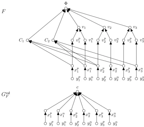
Proof. We start by showing part (A) of the theorem by devising a polynomial reduction from 3-SAT. Let Φ be a 3-CNF formula with clauses C1, . . . , Cmand variables x1, . . . , xn. In the following we construct a value-based system F = (X, A, V, η) whose value graph is a tree such that the query argument Φ ∈ X is subjectively accepted in F if and only if the formula Φ is satisfiable.
• The query argument Φ; • Seven arguments vi, vni, v p i, xni, x p i, yin, and y p i for every 1 ≤ i ≤ n; • One argument Cjfor every 1 ≤ j ≤ m.
The set A contains the following attacks:
• Three attacks (vi, Φ), (vip, vi), and (vin, vi) for every 1 ≤ i ≤ n; • One attack (Cj, Φ) for every 1 ≤ j ≤ m;
• Four attacks (xpi, vpi), (xni, v n i), (y p i, x p i), and (y n i, x n i) for every 1 ≤ i ≤ n; • One attack (xpi, Cj) for every clause Cjwhere the variable xioccurs positively; • One attack (xn
i, Cj) for every clause Cjwhere the variable xioccurs negatively. The set V contains the following values:
• One value c for the arguments in X \ { xn i, x p i, y n i, y p
i | 1 ≤ i ≤ n }, i.e., η(x) = c if and only if x ∈ X \ { xni, xpi, yin, yip| 1 ≤ i ≤ n }; • Four values xn i, x p i, y n i, y p
i for every 1 ≤ i ≤ n such that η(x) = x if and only if x ∈ { xn i, x p i, y n i, y p i | 1 ≤ i ≤ n }.
F
Φ C1 C2 v1 v2 v3 v1p vn 1 v p 2 v n 2 v p 3 v n 3 xp1 xn 1 x p 2 x n 2 x p 3 x n 3 y1p yn 1 y p 2 y n 2 y p 3 y n 3G
val F c xp1 xn 1 x p 2 x n 2 x p 3 x n 3 y1p yn1 y2p yn2 y3p yn3Figure 1. Illustration for the reduction used in the proof of Theorem 1, showing the AF F together with it’s value graph Gval
F, obtained from the 3-CNF formula φ = C1∧ C2with C1= x1∨ x2∨ x3and C2= ¬x1∨ x2∨ ¬x3.
An illustration for the VAF F and it’s value graph is given in Figure 1. It is not difficult to see that the value graph Gval
F of the constructed value-based system is a tree and that the VAF F can be constructed from Φ in polynomial time.
To establish part (A) of the theorem it remains to show that the formula Φ is satisfiable if and only if the argument Φ is subjectively accepted in F .
Suppose that the formula Φ is satisfied by an assignment β. We consider a specific audience ≤ defined as:
• η(ypi) < η(xpi) and η(yn
i) > η(xni) whenever β(xi) = true; • η(ypi) > η(xpi) and η(yn
i) < η(xni) whenever β(xi) = false.
Because F≤is acyclic it has a unique preferred extension GE(F≤) which using Proposition 1 is equal to IN (Λ(F≤)). We need to show that the argument Φ is labeled IN by the labeling Λ(F≤). Because β assigns a value to every variable of the formula Φ it follows that for every 1 ≤ i ≤ n one of the arguments xpi and xni is labeled IN and the other is labeled OUT , and Λ(F≤)(xpi) = IN if and only if β(xi) = true. Hence, for every 1 ≤ i ≤ n one of the arguments vipand v
n
i is labeled IN by Λ(F≤) (Λ(F≤)(vpi) = IN if and only if Λ(F≤)(x
p
i) = OUT ) and hence the argument viis labeled OUT by Λ(F≤). Furthermore, because the assignment β satisfies the formula Φ we know that every argument Cj is attacked by some argument x ∈ { xpi, xni | 1 ≤ i ≤ n } such that Λ(F≤)(x) = IN and hence Λ(F≤)(Cj) = OUT for every 1 ≤ j ≤ m. But then the argument Φ is labeled IN by Λ(F≤) and Φ ∈ GE(F≤).
To see the reverse direction suppose that the argument Φ is subjectively accepted in F and let ≤ be a specific audience of F witnessing this. Again using Proposition 1 we know that an argument is contained in the unique preferred extension of F≤ if and only if the argument is labeled IN by Λ(F≤). We will first show that for every 1 ≤ i ≤ n there is at most one argument x ∈ {xni, x
p i} such that η(x) > c and Λ(F≤)(x) = IN . Suppose this is not the case, i.e., there is some 1 ≤ i ≤ n such that η(xni), η(x
p
i) > c and Λ(F≤)(x n
i) = Λ(F≤)(xpi) = IN . It follows that both arguments vn
i and v p
i are labeled OUT by Λ(F≤) and hence Λ(F≤)(vi) = IN . But then Λ(F≤)(Φ) = OUT contradicting the assumption that the argument Φ is contained in the unique preferred extension of F≤. We will now show that the assignment β with β(xi) = true if η(xpi) > c and Λ(F≤)(x
p i) = IN and β(xi) = false otherwise is a satisfying assignment for the formula Φ. Again suppose not. Then there is a clause Cjthat is not satisfied by the assignment β. Let xibe a variable contained in Cj. If xi is contained positively in Cjthen β(xi) = false and consequently either η(xpi) < c or Λ(F≤)(xpi) = OUT . Similarly, if xi is contained negatively in Cj then β(xi) = true and consequently either η(xn
i) < c or Λ(F≤)(xni) = OUT . It follows that either η(x) < c or Λ(F≤)(x) = OUT for every argument that could attack the argument Cj in F≤ and hence Λ(F≤)(Cj) = IN . Hence, Λ(F≤)(Φ) = OUT contradicting the assumption that the argument Φ is contained in the unique preferred extension of F≤.
To prove part (B) of the theorem, we modify F into F0 by adding the argument Φ0 and the attack (Φ, Φ0) to F . The value of Φ0 in F0is set to c. Since Φ is the only attacker of Φ0, the target argument Φ0is objectively accepted in F0if and only if Φ is not subjectively accepted in F0. Because of the construction of F0 we have that the argument Φ is subjectively accepted in F0if and only if it is subjectively accepted in F . Hence (using part (A) of the theorem) it follows that the argument Φ0 is objectively accepted in F0 if and only if the formula Φ is not satisfiable. This completes the proof.
4. An Algorithm for Bounded Treewidth
In this section we present the dynamic programming algorithm and establish our tractability results. Let F = (X, A, V, η) be a VAF, x1 ∈ X, and (T, χ, r) a nice tree decomposition of width at most w of GvalF. For t ∈ V (T ), let Xtdenote the set η−1(χ(t)). Allowing a slight abuse of notations, we denote the set δ−F(Xt) := { x ∈ Xt | (y, x) ∈ A and y ∈ Nt} by δ−(t) and call it the incoming border of t. Likewise we denote the set δ+F(Xt) by δ+(t), which is called the outgoing border of t. The border δ(t) of t is the union δ(t) = δ+(t) ∪ δ−(t). incoming border of t, denoted δ+(t), to be δ+(t) = { x ∈ η−1(χ(t)) | (y, x) ∈ A and y ∈ N
t}. The outgoing border δ−(t) of t is the set δ−(t) = { x ∈ η−1(χ(t)) | (x, y) ∈ A and y ∈ Nt}. The border δ(t) of t is the union δ(t) = δ+(t) ∪ δ−(t). Our main tractability result states that for each fixed value ∆ := max
t∈V (T )|δ(t)| and fixed treewidth w, both ACCEPTANCEproblems can be solved in uniformly polynomial time. Theorem 2. Given a VAF F = (X, A, V, η), an argument x1 ∈ X, and a nice tree decomposition (T, χ, r) of width at most w for Gval
ACCEPTANCEandOBJECTIVEACCEPTANCEcan be solved in timeO(2∆·(2∆(w+1)!)2·(vw(F )+ aw(F )) · |V |).
We establish the above theorem with a dynamic programming algorithm over the given nice tree decomposition. The algorithm computes a set of so-called records (compact representations of pos-sibly preferred extensions) for each node of the tree decomposition in a bottom-up manner. A record of a tree node t ∈ V (T ) is a triple R = (I, O, ≤) such that:
1. I ⊆ δ−(t); 2. O ⊆ δ+(t);
3. ≤ is a specific audience for F [χ(t)].
Let t ∈ V (T ), R = (I, O, ≤) a record of t and ≤ta specific audience for F [χ∗(t)] that is compatible with ≤. We define the propagation of R as Λ(R) = Λ(σ(F≤[χ(t)], O)) and the propagation of R with respect to ≤tas Λ≤t(R) = Λ(σ(F≤t[Nt], α≤t(I, Nt))). We say that R = (I, O, ≤) represents
a specific audience ≤tfor F [χ∗(t)] if ≤tis compatible with ≤ and O = α≤t(IN (Λ≤t(R)), χ(t)).
We say that R = (I, O, ≤) is valid if there is an audience ≤tfor F [χ∗(t)] that is represented by R. With each tree node t ∈ V (T ) we associate the set R(t) of all valid records for t. Informally, if R is a valid record that represents a specific audience ≤tthen the set O contains exactly those arguments that are attacked by an argument that is labeled IN by Λ≤t(R) and the set I contains exactly those
arguments that are labeled IN by Λ(R) and attack arguments in Nt.
Lemma 2. Let t ∈ V (T ). Then for every I ⊆ δ−(t), and every specific audience ≤tforF [χ∗(t)] there is a recordR = (I, O, ≤) ∈ R(t) that represents ≤t.
Proof. The Lemma follows immediately from the definition of R(t).
The following four lemmas show that we can compute the set R(t) of all valid records for a tree node t from the sets R(t0) of all valid records for every child t0of t in T .
Lemma 3 (leaf node). Let t ∈ V (T ) be a leaf node of (T, χ). Then R = (I, O, ≤) ∈ R(t) if and only ifI = ∅, O = ∅ and ≤ is a specific audience of F [χ(t)]. Furthermore, the set R(t) can be computed in timeO((w + 1)!).
Proof. The Lemma follows because δ(t) = ∅ for every leaf node t ∈ V (T ).
Lemma 4 (join node). Let t ∈ V (T ) be a join node of (T, χ) and t1,t2be the children oft in T . Then R = (I, O, ≤) ∈ R(t) if and only if there are records R1 = (I1, O1, ≤1) ∈ R(t1) and R2= (I2, O2, ≤2) ∈ R(t2) such that the following conditions hold:
J1 I = I1∪ I2; J2 O = O1∪ O2; J3 ≤=≤1=≤2;
J4 I1∩ δ−(t1) ∩ δ−(t2) = I2∩ δ−(t1) ∩ δ−(t2)
Furthermore, the set R(t) can be computed from the sets R(t1) and R(t2) in time O(|R(t1)| · |R(t2)| · |δ(t)|.
Proof. We start with the following claim.
Claim 1. Let ≤t be a specific audience forF [χ∗(t)], ≤t1 a specific audience for F [χ
∗(t 1)], and ≤t2 a specific audience forF [χ
∗(t
2)] such that ≤tis compatible with≤t1 and≤t2. Furthermore,
letR = (I, O, ≤) be a record in R(t) that represents ≤t,R1= (I1, O1, ≤1) be a record in R(t1) that represents≤t1, andR2= (I2, O2, ≤2) be a record in R(t2) that represents ≤t2. IfR, R1, and
We first prove the equation IN (Λ≤t(R)) ∩ η
−1(N
ti) = IN (Λ≤ti(Ri)) ∩ η
−1(N
ti) for i =
1, 2 and w.l.o.g. let i = 1. Note that the condition J4 implies I ∩ δ−(t
1) = I1∩ δ−(t1). Due to Proposition 2, it follows that the two propagations Λ≤t(R) and Λ≤t1(R1) are identical on η
−1(N ti).
The equation is an immediate consequence.
Observe that for a valid record R = (I, O, ≤), x ∈ O if and only there exists y ∈ IN (Λ≤t(R))∩
η−1(Nt). Let x ∈ O and let y ∈ IN (Λ≤t(R)) ∩ η
−1(N
t). Due to the above equation, we have y ∈ IN (Λ≤t(R)) ∩ η −1(N t1 ∪ Nt2) = S2 i=1[IN (Λ≤ti(Ri)) ∩ η −1(N
ti)]. The validity of the
record Ri = (Ii, Oi, ≤i) implies x ∈ O1∪ O2. For the opposite direction, let x ∈ O1w.l.o.g and let y ∈ IN (Λ≤t1(R1)) ∩ η−1(Nt1). The above equations indicates IN (Λ≤t1(R1)) ∩ η
−1(N t1) ⊆
IN (Λ≤t(R)) ∩ η
−1(N
t) and it follows that x ∈ O. This completes the proof of the claim.
We now proceed to show the lemma. So suppose that R = (I, O, ≤) ∈ R(t). It follows that there is a specific audience ≤tfor F [χ∗(t)] that is represented by R. For every 1 ≤ i ≤ 2, we set Ii= I ∩ δ−(ti), ≤i=≤, and ≤tito be the unique specific audience for F [χ
∗(t
i)] that is compatible with ≤t. Because of Lemma 2, there are records Ri = (Ii, Oi, ≤i) ∈ R(ti) that represent ≤ti.
Observe that R, R1, and R2satisfy the conditions J1, J3, and J4. Using Claim 1 we obtain that R, R1, and R2also satisfy the condition J2.
To see the reverse direction let 1 ≤ i ≤ 2 and suppose that there are records Ri = (Ii, Oi, ≤i ) ∈ R(ti) that satisfy the conditions J3 and J4. It follows that each Rirepresents a specific audiences ≤tifor F [χ
∗(t
i)]. Let I = I1∪ I2, ≤=≤1and ≤tbe the unique specific audience for F [χ∗(t)] that is compatible with ≤t1and ≤t2. Because of Lemma 2 it holds that there is a record R = (I, O, ≤) ∈
R(t) that is represented by ≤t. Observe that the records R, R1and R2already satisfy the conditions J1, J3, and J4. It now follows from Claim 1 that they also satisfy condition J2.
It remains to show that R(t) can be computed from R(t1) and R(t2) in time O(|R(t1)|·|R(t2)|· |δ(t)|). Using the first statement of the lemma it follows that R(t) can be computed from R(t1) and R(t2) by applying the following steps to every pair (R1= (I1, O1, ≤1) ∈ R(t1), R2= (I2, O2, ≤2 ) ∈ R(t2)) of records:
1. Check whether R1 and R2satisfy condition J4 and ≤1 is compatible with ≤2. If not then reject the pair (R1, R2), if they do, proceed to step 2.
2. Compute the record R from R1and R2 according to the conditions J1–J3 and store R in R(t).
Because the steps 1. and 2. can be carried out in time O(|δ(t)|) it follows that the overall running time to compute R(t) from R(t1) and R(t2) is O(|R(t1)| · |R(t2)| · |δ(t)|).
Lemma 5 (introduce node). Let t ∈ V (T ) be an introduce node of (T, χ) with child t0, such that χ(t) = χ(t0) ∪ {v0}. Then R = (I, O, ≤) ∈ R(t) if and only if there is a record R0= (I, O, ≤0) ∈ R(t0) such that ≤0 is compatible with≤. Furthermore, the set R(t) can be computed from the set R(t0) in time O(|R(t0)| · (w + 1)).
Proof. So suppose that R = (I, O, ≤) ∈ R(t). It follows that R represents a specific audience ≤t for F [χ∗(t)]. Let ≤0be the unique specific audience for F [χ(t0)] that is compatible with ≤t. Because of Lemma 2 it follows that there is a record R0 = (I, O0, ≤0) ∈ R(t0) that represents ≤t. Using Proposition 3 we obtain O = O0.
To see the reverse direction suppose that there is a record R0= (I0, O0, ≤0) ∈ R(t0). It follows that R0represents a specific audience ≤t0 for F [χ∗(t0)]. Let ≤ be any specific audience for F [χ(t)]
that is compatible with ≤t0 and let ≤tbe any specific audience for F [χ∗(t)] that is compatible with
both ≤t0 and ≤. Because of Lemma 2 it follows that there is a record R = (I0, O, ≤) ∈ R(t0) that
represents ≤t. Using Proposition 3 we obtain O = O0.
It remains to show that R(t) can be computed from R(t0) in time O(|R(t1)| · (w + 1)). Using the first statement of the lemma it follows that we can compute R(t) from R(t0) by computing one record R = (I0, O0, ≤) for every record R0 = (I0, O0, ≤0) ∈ R(t0) and every specific audience ≤ for F [χ(t)] that is compatible with ≤0. Observe that there are at most w + 1 specific audiences ≤ for F [χ(t)] that are compatible with a specific audience ≤0 for F [χ(t0)] and the record R can be
computed from R0 and ≤ in time O(1). It follows that the overall running time to compute R(t) from R(t0) is O(|R(t0)| · (w + 1)).
Lemma 6 (forget node). Let t be a forget node of (T, χ) with child t0such thatχ(t) = χ(t0) \ {v0}. ThenR = (I, O, ≤) ∈ R(t) if and only if there is a set S ⊆ δ−(t) \ δ−(t0) and a record R0 = (I0, O0, ≤0) ∈ R(t0) such that: F1 I = (I0\ P ) ∪ S; F2 P = IN (Λ(Fv0)) ∩ δ −(t0); F3 O = (δ+(t) ∩ O0) ∪ α ≤0(IN (Λ(Fv 0)), χ(t)); F4 ≤ is compatible with ≤0; whereP = I0∩η−1(v 0) and Fv0 = σ(F [v0], (η −1(v
0)∩O0)∪α≤0(I, v0)). Furthermore, the set R(t)
can be computed from the setR(t0) in time O(2|δ−(t)\δ−(t0)|
·|R(t0)|·(|η−1(v
0)|+|A(F [v0])|+∆)).
Proof. So suppose that R = (I, O, ≤) ∈ R(t). It follows that R represents a specific audience ≤t for F [χ∗(t)] = F [χ∗(t0)]. Let S = I ∩ (δ−(t) \ δ−(t0)), P = IN (Λ≤t(R)) ∩ η
−1(v
0) ∩ δ−(t0), I0 = I \ S ∪ P , and ≤0 be a specific audience for F [χ(t0)] that is compatible with ≤t. It follows from Lemma 2 that there is a record R0 = (I0, O0, ≤0) ∈ R(t0) that represents ≤t. Consequently, the records R, R0, and S satisfy F1 and F4. Because Λ(Fv0) is compatible with Λ≤t(R) we obtain
that R, R0and S also satisfy F2 and F3.
To see the reverse direction suppose that there is a record R0 = (I0, O0, ≤0) ∈ R(t0), a set S ⊆ (δ−(t) \ δ−(t0)) and a record R = (I, O, ≤) of t that satisfy F1–F4. It follows that there is a specific audience ≤t0 for F [χ∗(t0)] = F [χ∗(t)]. We show that R represents ≤t0 and hence R ∈ R(t). Let
FL= σ(σ(F≤t0[Nt], α≤t0(I, Nt0), s1), α≤t0(I, v0), s2),, X1= Nt0 ∪ {s1}, X2= η −1(v 0) ∪ {s2}, F1 = σ(FL[X1], αFL(IL, X1), s1), F2 = σ(FL[X2], αFL(OL, X2), s2), OL = O 0 ∩ η−1(v 0), IL= P . Observe that by construction Λ(FL) is compatible with Λ≤t0(R), Λ(F1) is compatible with
Λ≤t0(R0), and Λ(F2) is compatible with Λ(Fv0). Hence, αFL(IN (Λ(F1)), X2) = O
0∩ η−1(v 0) = OLand because of F2 also IN (Λ(F2)) ∩ δ−FL(X2) = P = IL. It now follows from Lemma 1 that Λ(FL) = Λ≤t0(R) is compatible with Λ(F1) ∪ Λ(F2) = Λ≤t0(R0) ∪ Λ(Fv0). Consequently,
α≤t0(IN (Λ≤t0(R)), χ(t)) =α≤t0(IN (Λ≤t0(R0) ∪ Λ(Fv0)), χ(t)) =α≤t0(IN (Λ≤t0(R 0), χ(t)) ∪ α ≤t0(IN (Λ(Fv0))), χ(t)) =(δ+(t) ∩ O0) ∪ α ≤t0(IN (Λ(Fv0)), χ(t)) =(δ+(t) ∩ O0) ∪ α ≤0(IN (Λ(Fv 0)), χ(t)) =O
It follows that R represents ≤t0.
It remains to show that R(t) can be computed from R(t0) in time O(2|δ−(t)\δ−(t0)|· |R(t0)| · (|η−1(v0)| + |A(F [v0])| + ∆)) Because of the first statement of this lemma it follows that we can compute R(t) from R(t0) using the following procedure:
1. For every S ⊆ (δ−(t) \ δ−(t0)) and R0= (I0, O0, ≤0) ∈ R(t0) do 2. P = I0∩ η−1(v 0) 3. P0= IN (Λ(Fv0)) 4. if P == P0∩ δ−(t0) then 5. I = (I0\ P ) ∪ S 6. O = (δ+(t) ∩ O0) ∪ α≤0(P0, χ(t))
7. ≤ is the unique specific audience for F [χ(t)] that is compatible with ≤0
Because there are at most 2|δ−(t)\δ−(t0)| sets S ⊆ (δ−(t) \ δ−(t0)) and exactly |R(t0)| records in R(t0) we obtain that everything inside the initial for-loop is executed at most 2|δ−(t)\δ−(t0)|
· |R(t0)| times. We obtain the following worst-case running time for the lines 2.–9.:
2. O(|η−1(v0)|);
3. Because |X(Fv0)| ≤ |η
−1(v
0) + 1| and |A(Fv0)| ≤ |A(F [v0])| + |η
−1(v
0)| it follows from Proposition 1 that P0can be computed in time O(|η−1(v0)| + (|A(F [v0])| + |η−1(v0)|)) ⊆ O(|η−1(v0)| + |A(F [v0])|);
4. Because |P | ≤ |η−1(v0)| we can check whether P is equal to P0 ∩ δ+(t0) in time O(|η−1(v0)|);
5. O(|δ−(t)|) ⊆ O(∆);
6. O(|δ+(t0)| + |δ+(t)|) ⊆ O(∆); 7. O(1);
8. O(1).
It follows that the overall running time to compute R(t) from R(t0) is O(2|δ−(t)\δ−(t0)|· |R(t0)| · (|η−1(v0)| + |A(F [v0])| + ∆)).
We say that a record R = (I, O, ≤) ∈ R(r) is realizable if I = (IN (Λ(R)) ∩ δ−(r)). We say that a record R = (I, O, ≤) ∈ R(r) is compatible with a specific audience ≤F of F if Λ(R) is compatible with Λ(F≤F). The following lemma shows that the set of all realizable records in R(t)
is a complete representation of all specific audiences of F .
Lemma 7. Every specific audience ≤F ofF is compatible with some realizable record R ∈ R(r). Furthermore, every realizable recordR ∈ R(r) is compatible with some specific audience ≤FofF .
Proof. Suppose there is a specific audience ≤F for F . Let I = IN (Λ(F≤F)) ∩ δ
−(t) and ≤ a specific audience for F [χ(r)] that is compatible with ≤F. It follows from Lemma 2 that there is a record R = (I, O, ≤) ∈ R(r) that is represented by ≤F and O = α≤F(IN (Λ≤F(R)), χ(r)).
We first show that R is compatible with ≤F with the help of Lemma 1. Let FL = F≤F, X1 =
η−1(Nr), X2 = η−1(χ(r)), IL = I, and OL = O and let F1and F2be the AFs as defined in the statement of Lemma 1. Because R represents ≤F we have OL = α≤F(IN (Λ(F≤F[Nr])), χ(r)) =
αFL(IN (Λ(F1)), X2) and we also know that IL= IN (Λ(F≤F)) ∩ δ
−(t) = IN (Λ(F
L)) ∩ δF−L(X2).
Consequently, all pre-requisites of Lemma 1 are fulfilled and Λ(FL) = Λ(F≤F) is compatible with
Λ(F2) = Λ(R). But then R is also realizable because I = IN (Λ(F≤F)) ∩ δ
−(r) = IN (Λ(R)) ∩ δ−(r) as required.
To see the reverse direction suppose that R = (I, O, ≤) ∈ R(r) is realizable. Because R is valid it follows that there is a specific audience ≤F for F that is represented by R. We show that R is compatible with ≤Fwith the help of Lemma 1. Let FL= F≤F, X1= η
−1(N
r), X2= η−1(χ(r)), IL = I, and OL = O and let F1 and F2 be the AFs as defined in the statement of Lemma 1. Because R represents ≤F we have OL = α≤F(IN (Λ(F≤F[Nr])), χ(r)) = αFL(IN (Λ(F1)), X2)
and because R is realizable it follows that IL = IN (Λ(R)) ∩ δ−(t) = IN (Λ(F2)) ∩ δF−L(X2). Consequently, all pre-requisites of Lemma 1 are fulfilled and Λ(FL) = Λ(F≤F) is compatible with
Λ(F2) = Λ(R).
Lemma 8. Let R ∈ R(r). Then we can decide whether R is realizable and whether x1∈ Λ(R) in timeO(|X(F [η(x1)]| + |A(F [η(x1)])| + ∆).
Proof. Let R = (I, O, ≤) ∈ R(r). To decide whether R is realizable we need to compute Λ(R) = Λ(σ(F≤[χ(r)], O) = Λ(σ(F [η(x1)], O)). Because of Proposition 1 this can be done in time O(|η−1(η(x1))| + |A[η(x1)]| + ∆). Once we have computed Λ(R) we can check whether R is realizable and whether x1 ∈ IN (Λ(R)) in time O(∆). Hence, both problems can be decided in time O(|η−1(η(x1))| + |A[η(x1)]| + ∆).
Proof of Theorem 2. Let F = (X, A, V, η) be the given VAF, x1 ∈ X the query argument, and (T, χ, r) the nice tree decomposition of width at most w for Gval
F such that |T | = O(|V |) and χ(r) = {η(x1)}. Starting from the leaf nodes of the nice tree decomposition the algorithm computes the set of all valid records for each tree node t ∈ V (T ) in a bottom-up manner. Denote by Rmax= maxt∈V (T )|R(t)|. Combining the running times for a leaf node of O((w + 1)!) (Lemma 3), for a join node of O(|R(t1)| · |R(t2)| · |δ(t)|) ⊆ O((Rmax)2· ∆) (Lemma 4), for an introduce node of O(|R(t0)| · (w + 1)) ⊆ O(Rmax· (w + 1)) (Lemma 5), and for a forget node of O(2|δ
−(t)\δ−(t0)|
· |R(t0)| · (|η−1(v
0)| + |A(F [v0])| + ∆)) ⊆ O(2∆· Rmax · (vw(F ) + aw(F ) + ∆)) (Lemma 6) we obtain O(2∆· (Rmax)2· (w + 1)! · (vw(F ) + aw(F ) + ∆)) as the worst-case running time of the algorithm for a tree node t ∈ V (T ). Because there at most O(|V |) tree nodes in T we obtain O(2∆· (Rmax)2· (w + 1)! · (vw(F ) + aw(F ) + ∆) · |V |) as the running time that our algorithm needs to compute the sets of all valid records for every tree node t ∈ V (T ).
It follows from Lemma 7 that the argument x1is subjectively accepted in F if and only if there is a realizable record R ∈ R(r) such that x1 ∈ IN (Λ(R)). For the same reason, the argument x1 is objectively accepted in F if and only if for all realizable records R ∈ R(r) it holds that x1 ∈ IN (Λ(R)). Because there are at most 2∆records in R(r) and for each such record R we can check whether R is realizable and whether x1 ∈ IN (Λ(R)) in time O(|X(F [η(x1)]| + |A(F [η(x1)])| + ∆) ⊆ O(vw(F ) + aw(F ) + ∆) (see Lemma 8) it follows that given R(r), we can decide whether x1is subjectively or objectively accepted in F in time O(2∆· (vw(F ) + aw(F ) + ∆)). Combining these two steps leads to an overall running time of the algorithm of O(2∆· (R
max)2· (w + 1)! · (vw(F ) + aw(F ) + ∆) · |V |). It remains to observe that |Rmax| ≤ 2∆· (w + 1)!
References
[1] P. Baroni and M. Giacomin. Semantics of abstract argument systems. In I. Rahwan and G. Simari, editors, Argumen-tation in Artificial Intelligence, pages 25–44. Springer Verlag, 2009.
[2] T. J. M. Bench-Capon. Persuasion in practical argument using value-based argumentation frameworks. J. Logic Comput., 13(3):429–448, 2003.
[3] T. J. M. Bench-Capon and P. E. Dunne. Argumentation in artificial intelligence. Artificial Intelligence, 171(10-15):619– 641, 2007.
[4] P. Besnard and A. Hunter. Elements of Argumentation. The MIT Press, 2008.
[5] H. L. Bodlaender. A linear-time algorithm for finding tree-decompositions of small treewidth. SIAM J. Comput., 25(6):1305–1317, 1996.
[6] A. Bondarenko, P. M. Dung, R. A. Kowalski, and F. Toni. An abstract, argumentation-theoretic approach to default reasoning. Artificial Intelligence, 93(1-2):63–101, 1997.
[7] P. M. Dung. On the acceptability of arguments and its fundamental role in nonmonotonic reasoning, logic programming and n-person games. Artificial Intelligence, 77(2):321–357, 1995.
[8] P. E. Dunne. Computational properties of argument systems satisfying graph-theoretic constraints. Artificial Intelli-gence, 171(10-15):701–729, 2007.
[9] P. E. Dunne. Tractability in value-based argumentation. In P. Baroni, F. Cerutti, M. Giacomin, and G. R. Simari, editors, Computational Models of Argumentation, Proceedings of COMMA 2010, volume 216 of Frontiers in Artificial Intelligence and Applications, pages 195–206. IOS, 2010.
[10] P. E. Dunne and T. J. M. Bench-Capon. Complexity in value-based argument systems. In J. J. Alferes and J. A. Leite, editors, Logics in Artificial Intelligence, 9th European Conference, JELIA 2004, Lisbon, Portugal, September 27-30, 2004, Proceedings, volume 3229 of Lecture Notes in Computer Science, pages 360–371. Springer Verlag, 2004. [11] V. Gogate and R. Dechter. A complete anytime algorithm for treewidth. In Proceedings of the Proceedings of the
Twentieth Conference Annual Conference on Uncertainty in Artificial Intelligence (UAI-04), pages 201–208, Arlington, Virginia, 2004. AUAI Press.
[12] E. J. Kim, S. Ordyniak, and S. Szeider. Algorithms and complexity results for persuasive argumentation. Artificial Intelligence, 175:1722–1736, 2011.
[13] T. Kloks. Treewidth: Computations and Approximations. Springer Verlag, Berlin, 1994.
[14] S. Parsons, M. Wooldridge, and L. Amgoud. Properties and complexity of some formal inter-agent dialogues. J. Logic Comput., 13(3):347–376, 2003.
[15] J. L. Pollock. How to reason defeasibly. Artificial Intelligence, 57(1):1–42, 1992.