Development of a Probabilistic Framework for Debris Transport and Hazard
Assessment in Tsunami-Like Flow Conditions
Jacob Stolle1, Ioan Nistor2, Nils Goseberg3, and Emil Petriu4 1
Centre Eau Terre Environnement, INRS, 490 Rue de la Couronne, Québec, Québec, Canada, G1K 9A9, [email protected] (https://orcid.org/0000-0003-0902-9339)
2 Department of Civil Engineering, University of Ottawa, 161 Louis Pasteur Drive, Ottawa, ON, Canada, K1N 6N5,
[email protected] (https://orcid.org/0000-0001-8436-4781)
3 Leichtweiß-Institute for Hydraulic Engineering and Water Resources, Technische Universität Braunschweig, Beethovenstraße
51a, 38106 Braunschweig, Germany, [email protected] (https://orcid.org/0000-0002-1550-3001)
4 School of Electrical Engineering and Computer Science, 800 King Edward Avenue, Ottawa, ON, Canada, K1N 6N5,
Abstract
Past hydraulic and structural design has predominantly used deterministic methods, often neglecting the stochastic nature that underlies transient loading processes. Nowadays, probabilistic design methods have gained wider attention. The accurate estimates of design conditions for structures need to consider the probabilistic properties of the loads. One of the more challenging loads in extreme flooding events is related to debris transport and loading during hydrodynamic hazardous events. While crucial to assess damage on infrastructure as part of the design cycle, field surveys and numerical modeling provide little guidance as to how the motion of debris within these natural disasters can be adequately captured. The study presented herein examines an idealized case regarding the transport of debris entrained during extreme flooding events by evaluating the characteristics of shipping containers motion entrained in a dam-break flow over a flat, horizontal bed. In aiding the promotion of probabilistic methods, this study proposes characteristics of the stochastic properties of debris transport, focussing on the lateral displacement and velocity of debris based on the experimental results. The magnitude of the lateral displacement was shown to strongly correlate with the local hydrodynamic conditions and the initial configuration of the debris. The results of the physical model were then incorporated into a probabilistic framework. The aim for developing this framework is to facilitate debris hazard assessment in extreme flooding event studies.
Keywords: Debris; Flood; Tsunami; Natural Hazards; Stochastic; Physical Modelling
1
Introduction
1.1 Background
The extent of the damage caused by the 2011 Tohoku Tsunami demonstrated that state-of-the-art coastal protection measures and disaster mitigation strategies do not adequately address the vulnerability of coastal communities. In the case of the 2011 Tohoku Tsunami, the Japanese government had historically used a deterministic tsunami hazard assessment (Macabuag et al. 2018). However, historical records for the tsunamis affecting the Tohoku region did not comprise an event large enough to realistically estimate the true potential of the tsunami hazard (Mori et al. 2011). In an attempt to address this design issue, the ASCE 7 Chapter 6 – Tsunami Loads and Effects (ASCE 2016) introduced the first tsunami-specific standard written in mandatory language that addresses tsunami hazard from a probabilistic perspective (Chock 2016). The probabilistic analysis presented in this document was performed by developing a large data set of tsunami wave scenarios based on the different source mechanisms (i.e. slip area, extent of rupture). The standard then uses either an Energy Grade Line (EGL) method (Kriebel et al. 2017) or recommends using a numerical model to determine on-shore flow conditions (water depth and velocity). While the ASCE7 Chapter 6 prescribed a probabilistic approach to tsunami hazard assessment, the probabilistic approach was restricted to flow conditions. Other aspects, such as debris and scour, were so far not placed within the context of a probabilistic framework, although these factors may result in very
large design loads, often governing the entire structural design. Excluding a probabilities approach from assessing the debris and scour effects was primarily because of limited available research towards assessing these effects from a probabilistic perspective (Nistor et al. 2017). To address debris hazard, two critical aspects to consider are (1) the likelihood that debris, or a multitude of debris, will impact a given structure and (2) the magnitude of the debris impact force. Considering the single degree-of-freedom model commonly used within design standards (Haehnel and Daly 2004, Nistor et al. 2017), the impact force of debris onto a rigid vertical structure can be derived as follows:
𝐹𝐹 = 𝑢𝑢�𝑘𝑘𝑑𝑑𝑚𝑚𝑑𝑑 (1)
where 𝑢𝑢 is the velocity immediately before impact, 𝑘𝑘𝑑𝑑 is the stiffness of the debris, and 𝑚𝑚𝑑𝑑 is the mass of the debris. The magnitude of the debris impact force for a single type of debris (same mass and stiffness) is dictated by the impact velocity. Eq. (1) represents the maximum potential impact force on a structure as it assumes that the structure is directly impacted and that it does not displace/deform to absorb a portion of the energy (Stolle et al. 2019). Additionally, the impact geometry can significantly influence the impact force (Derschum et al. 2018).
The ASCE7 Chapter 6 (2016) approached debris hazard assessment in deterministic fashion, using two different methods depending on the buildings risk category, inundation depth, flow velocity and proximity to a debris source. In all cases, impact velocity was prescribed as the maximum local flow velocity. In the ASCE7 Chapter 6, the local flow velocity and water depth are calculated using information obtained from the probabilistic tsunami hazard maps. For all buildings within the 0.914 m inundation depth (considered the maximum depth debris would still float), buildings need to be designed for impact on structural members for small, common debris, such as floating wooden logs and construction material. For building close to a source of large debris, such as shipping containers and barges, buildings needed to be designed for “extraordinary” impact.
The requirement to design for “extraordinary” debris impacts was based on a field study conducted in the aftermath of the 2011 Tohoku Tsunami which examined the dispersal of shipping containers and ships in four flooded regions along the Japanese coast (Naito et al. 2014). The methodology prescribed a spatial spreading of the debris originating from the geometric center of the debris source. The spreading extent was defined in the direction of tsunami inundation flow with a +/-22.5o spreading angle enclosing an area equal to 50 times the plan area of the debris. As such, any structure located within the enclosed area, and still within the 0.914 m inundation depth, requires “extraordinary” debris impact design. This angle was selected as a conservative estimation of the debris spreading based on their final resting position, with a known originating source.
While the Naito et al. (2014) approach represents a conservative estimation, as it captures the influence of multiple waves as well as the cyclical nature of the inundation and drawdown, the model cannot capture the probabilistic nature of debris dynamics as well as the intermediate steps (such as trajectory and velocity) necessary to assess the magnitude of debris impact forces. Their approach also does not reflect the physical processes involved in debris transport. Nistor et al. (2016) showed that as the number of pieces of debris increase (and therefore the plan area), the displacement of the debris in the flow direction decreases and the lateral displacement of the debris increases. As the Naito et al. (2014) approach holds the spreading angle constant, as the number of pieces of debris increases, the displacement in the flow direction increases. In addition, Goseberg et al. (2016) noticed that the built environment altered less significantly the spreading angle of debris, whereas inland distance of the transport process was influenced to a major extend by buildings. However, this study was performed under a limited number of building configurations at small-scale and found that the influence of the built environment depends heavily on direct debris-building interactions. Further research is necessary to address the influence of complex flow obstructions on debris transport.
For smaller debris, several probabilistic models have been proposed based on the surrounding environment. Reese et al. (2011), based on empirical analysis from the 2009 Samoan Tsunami, incorporated debris impact into fragility analysis by separately assessing buildings with clear debris impact features (i.e., debris lodged in the structure). However, they noted that this method was not sufficient alone as structures impact by debris were unlikely to have minor damage, therefore, not capturing the full range of damage states. Charvet et al. (2015) developed a method for including debris impact within fragility analysis by considering any building that collapses as a source of debris. The method selected a radius for debris transport (between 10 – 150 m), based on the fit of the model using multinomial logit regression, where any building within the selected radius was considered to be impacted by debris. Hatzikyriakou and Lin (2017), examining structural vulnerability under storm surge conditions, were able to estimate the vulnerability of a building, depending on the performance of the structures directly seaward. If the structures immediately seaward of the structure survived, they shielded the subsequent structures, however, if they failed, the resulting waterborne debris resulted in increased damage states.
Lin and Vanmarcke (2010) developed a theoretical risk analysis model that examined the transport of wind-borne debris. The model examined three key aspects related to debris transport: the generation, displacement, and velocity of the debris. The type of distribution used in each aspect was based on analysis of physical modelling experiments, with the mean behaviour informed by the physical behaviour of the debris. The present study intends to build upon the framework outlined in Lin and Vanmarcke (2010) and apply this framework to “extraordinary” debris impacts in flood-like events using results obtained from physical modelling. Debris hazard assessment has important applications in the design of flood-resistant structures (Chock 2016) and fragility analysis (Charvet et al. 2015) while also potentially informing recovery of valuable objects efforts in the aftermath of flooding events. With the overall aim of developing a stochastic framework for estimating debris hazard, the specific objectives of this study are:
• Based on previous state-of-the-art literature, develop an understanding of the parameters governing debris transport.
• Establish a methodology, based on physical processes, for estimating the displacement of the debris both in the flow direction and laterally.
• Develop a method for estimating the design loading conditions through the physical behaviour of debris motion.
This study focuses on applying the framework in tsunami-like flow conditions, in this case, a dam-break wave. The physical model was designed as an idealized, flat topography to limit the influence of aspects, such as bed slope and obstacles within the flow. In order to test and build the framework, the study will address one type of positively buoyant debris, scaled-down shipping containers, scaled considering Froude similitude.
2
Methodology
2.1 Experimental Facilities
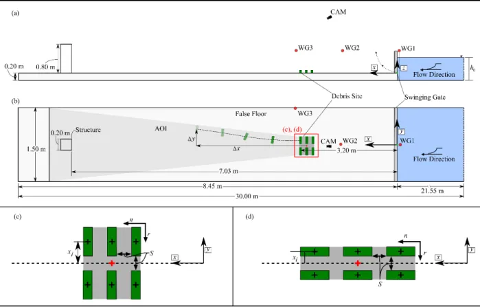
The physical modelling was performed in the Dam-break Flume at the University of Ottawa, Canada (Figure 1). This facility is 30 m long, 1.5 m wide, and 0.8 m deep, with a false floor 8.45 m long, 0.20 m high placed at one end of the flume. The remainder of the flume was used as a reservoir to impound a volume of water, which was released by a rapidly-opening swinging gate (Häfen et al. 2018, Stolle et al. 2018b). The coordinate system of the facility is defined from the upstream side of the gate on the bed of the false floor. The positive x-axis is in the direction of the flow, the positive y-axis is flume right, and the positive z-axis in the upwards direction.
Figure 1. University of Ottawa Dam-break Flume (30 m × 1.5 m × 0.8 m) side view (a) and top view (b). The red circles indicate the position of the wave gauges and the green box indicates the position of the debris. The faded grey trapezoid in (b) represents the area of interest used for debris tracking by CAM. The layouts of the debris site are shown in (c) and (d). The red cross represents the geometric center of the debris site. The parameters for the debris configuration are shown in (c) for orientation (Θ) = 0o
and (d) 90o.
The debris used in this experiment were 1:40 geometrically scaled shipping containers (0.15 m × 0.06 m × 0.06 m); made of high molecular weigh polyethylene (PE-HMW). The shipping containers were scaled as the mean weight of fully-loaded shipping container (Knorr and Kutzner 2008), considering Froude similitude (𝑚𝑚𝑑𝑑 = 0.236 +/- 0.005 kg). The resulting density (𝜌𝜌𝑑𝑑) and draft of the containers was approximately 416 kg/m3 and 0.025 m, respectively. The debris were placed with the centroids of the furthest downstream debris at x = 3.20 m. The number and configuration of the debris were varied throughout the experiment to examine the influence of the initial entrainment of the debris on debris transport, the configurations are outlined in Section 2.4. Before each experiment, the debris were sealed and covered in petroleum jelly for preventing water intrusion.
The experiments were performed within the context of a larger experimental protocol examining debris impact forces on a structure (Derschum et al. 2018, Stolle et al. 2018a, 2018c, 2019). The structure (0.20 m × 0.20 m × 0.80 m) was placed at a distance of 7.03 m from the gate. To eliminate potential interference from the structure, as well as from the reflected wave, the motion of the debris was tracked only to a distance of 6.50 m downstream of the gate, resulting in a maximum longitudinal displacement (∆𝑥𝑥) of 3.30 m. The debris continued to be displaced by the flow until captured in a net placed over the bottom drain of the flume.
The bed of the false floor was covered with 1 mm-sieved sand and painted to have a fixed bed surface. Stolle et al. (2018b), in a hydrodynamic analysis of the same flume, determined that the approximate Darcy-Weisbach friction factor was 0.0293 by fitting the instantaneous wave profile of various impoundment depths to the Chanson (2006) solution for a dam-break wave. The coefficient of static
friction (𝜇𝜇0) between the debris model and the false floor was approximately 0.40 (Stolle et al. 2018c), which slightly exceeds the suggested coefficient (0.30) used in the design of shipping container transportation methods (GDV 2003).
2.2 Instrumentation
Three wave gauges (WG, RBR WG-50, capacitance-type, accuracy = +/- 0.1%, 0.50 m measurement range, 1200 Hz) were placed in the flume (Figure 1). Wave gauge (WG1) was placed in the reservoir (at x = -0.10 m) to determine the opening of the gate. When the water surface in the reservoir dropped to 2% of the initial impoundment depth (h0), the gate was considered to be completely open, indicating thus the
start of each individual experiment (reference time, t = 0.00 s). Wave gauges WG2 and WG3 were placed on the false floor, z = 0.005 m above the bed at distances of x = 2.00 m and 3.20 m, to measure the propagation of the wave downstream. Before the WGs were placed in the flume, they were calibrated ensuring an R2 value of 0.99.
The debris were tracked through the area-of-interest using a high-definition camera (CAM, Basler pi1900-32gc). The CAM was externally triggered using a 25-Hz output signal from a data acquisition system (DAQ, National Instruments USB-6009). The signal was simultaneously sampled by a second DAQ system (HBM MX1601B), also sampling the WGs, to synchronize the images with the hydrodynamic data. The estimated synchronization error was approximately +/- 0.04 s.
2.3 Debris Tracking
The positions of the debris were tracked using a camera-based tracking algorithm (Stolle et al. (2016), through the area of interest (shown by the faded grey trapezoid in Figure 1(b)). However, the algorithm had to be adapted and modified for the purpose of this study. As noted in Stolle et al. (2016), the algorithm has difficulties tracking more than six debris of the same colour throughout image sequences. This is due to the algorithm passing the identifiers of the individuals between debris. As a result, the algorithm cannot reliably distinguish the trajectory of a single debris across the area of interest. As outlined in Stolle et al. (2016), the algorithm was separated into two distinct features: object detection and object tracking. The object tracking feature was mainly responsible for maintaining the unique identifier. As in this study up to 12 debris were used, the object tracking feature was eliminated to avoid challenges related to the passing of identifiers. The object detection algorithm was then used to identify the position of the centroid of the individual debris within each frame. The accuracy of the method without the object tracking algorithm was compared to manual selection of the individual debris within the image in three experimental trials resulting in an approximate error of +/- 0.045 m.
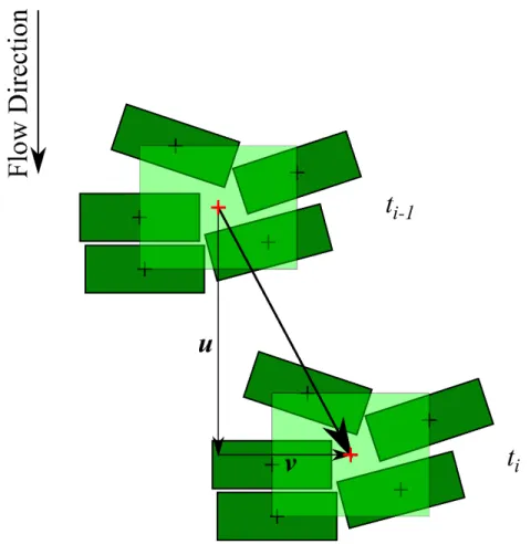
The challenge with removing the object tracking feature is the motion of the individual debris cannot be assessed. To address this issue in terms of the lateral displacement of the debris, the displacement discussed in the following section (∆𝑦𝑦) refers to the lateral displacement of each debris’ centroid (in each frame) from the geometric center of the initial configuration of the debris (at rest). The geometric center is determined based on the position of the centroid of each debris (represented by black crosses in Figure 2). The geometric center was determined by conceptualizing a rectangle that would capture the position of all the debris centroids in each image (green rectangle in Figure 2) and taking the mean of the outmost coordinates (red cross). Within this study, the initial geometric center was always positioned at y = 0.00 m. For the debris velocity, as the displacement of an individual debris could not be tracked, the velocity of the group of debris was assumed to be relatively constant. Therefore, the velocity of the group was calculated by the trajectory of the geometric center of the debris within each frame (Figure 2).
Figure 2. Measurement of debris position and velocity using the object detection algorithm (Stolle et al. 2016). The green box represents a single debris, the black crosses are centroids of individual debris, and the red crosses are the centroid of the debris group. The faded green box represents the conceptualized rectangle used in the determination of the centroid of the group.
2.4 Experimental Protocol
With the main objective of developing a probabilistic framework for debris dynamics which would be based on physical processes, dimensional analysis (Hughes 1993) was performed based on force balances (outlined in Section 3.1). To address the relevant parameters found through the dimensional analysis, several hydrodynamic forcing conditions and debris configurations were experimentally tested and used for the analysis (Table 1). The hydrodynamic forcing conditions was varied by changing the water depth impounded in the reservoir (ℎ0). The debris configuration was adjusted by changing the number of columns of debris (𝑟𝑟), the number of pieces of debris within each column (𝑛𝑛), the spacing between the edges of the debris (held constant in the x- and y-directions) (𝑆𝑆), and the orientation of the long axis of the debris (Θ). An Θ -value of 0o refers to the long axis of the debris perpendicular to the flow direction. Ten repetitions were performed per each experimental category for a total of 170 experimental tests.
Table 1. Experimental protocol. The experimental categories are named to represent the initial conditions. C – impoundment depth (h0), N – number of pieces of debris, R – number of columns of debris (r), S – debris spacing (S), O – debris orientation
(Θ). Experimental Category Impoundment Depth (ℎ0) [m] Number of Columns (𝑟𝑟) Number of pieces of Debris per Column (𝑛𝑛) Debris Spacing (𝑆𝑆) [m] Debris Orientation (Θ) [o] C20N1 R1S1O1 0.20 1 1 0 0
C40N1 R1S1O1 0.40 1 1 0 0 C40N1 R1S1O2 0.40 1 1 0 90 C20N3 R1S1O1 0.20 1 3 0.03 0 C40N3 R1S1O1 0.40 1 3 0.03 0 C20N6 R1S1O1 0.20 1 6 0.03 0 C20N6 R2S1O1 0.20 2 3 0.03 0 C40N1 R1S1O1 0.40 1 6 0.03 0 C40N1 R2S1O1 0.40 2 3 0.03 0 C50N6 R2S1O1 0.50 2 3 0.03 0 C20N12 R2S1O1 0.20 2 6 0.03 0 C20N12 R2S1O2 0.20 2 6 0.03 90 C40N12 R2S2O1 0.40 2 6 0.015 0 C40N12 R2S1O1 0.40 2 6 0.03 0 C40N12 R2S3O1 0.40 2 6 0.06 0 C40N12 R2S1O2 0.40 2 6 0.03 90 C50N12 R2S1O1 0.50 2 6 0.03 0
Before each experimental trial, excess water from the previous trial was removed from the flume bed. The debris were placed in the flume using set guides indicated on the bottom of the flume. The reservoir was filled to the set impoundment depth, wave absorbers were placed within the cross-section of the reservoir to aid in the attenuation of wave caused by the filling process. The impounded volume of water was released by operating the opening mechanism of the swing gate (Stolle et al. 2018b), entraining the debris and propagated them downstream. After each experiment, the debris were opened to remove any intrusion of water and were subsequently resealed with petroleum jelly.
3
Results
3.1 Dimensional Analysis
In determining the relevant parameters for flood-driven debris hazard, dimensional analysis (Hughes 1993) was performed examining results of previous literature. The dimensional analysis was performed assuming the propagation of debris over a flat, horizontal bed with no flow obstructions. The dependent parameter was the lateral displacement of the debris (∆𝑦𝑦).
Stolle et al. (2018c) showed that lateral spreading was dependent on the hydrodynamic forcing condition, therefore, the water depth (𝑑𝑑) and flow velocity (𝑐𝑐), and distance from the debris source (∆𝑥𝑥). Nistor et al. (2016) showed that the lateral spreading was a function of the number of pieces of debris present, Stolle et al. (2017) extended that work to show that it was dependent on the number of pieces of debris within each column of the initial configuration (𝑛𝑛) and the initial orientation of the debris (Θ). Stolle et al. (2018d) showed that the number of columns of the initial configuration (𝑟𝑟) and the spacing between the debris (𝑆𝑆) also dictated the extent of the lateral displacement. As the drag force acting on the debris dictates the influence of the hydrodynamic forcing condition on the debris motion (Shafiei et al. 2016),
the area exposed to the flow as defined by the characteristic length (𝑙𝑙) and viscosity (𝜇𝜇) plays a role. The initial entrainment of the debris is also critical in dictating the corresponding motion (Braudrick and Grant 2000, Rueben et al. 2014), the relative density of the debris (𝜌𝜌𝑑𝑑) and water (𝜌𝜌𝑤𝑤) as well as the gravitational constant (𝑔𝑔) and coefficient of friction (𝜇𝜇0) will also have an influence. Using the Buckingham pi-theorem, the resulting non-dimensional pi-groups were identified as:
∆𝑦𝑦 𝑑𝑑 = 𝑓𝑓 �Θ, 𝑛𝑛, 𝑟𝑟, ∆𝑥𝑥 𝑑𝑑 , 𝑆𝑆 𝑑𝑑 , 𝑙𝑙 𝑑𝑑 , 𝜌𝜌𝑑𝑑 𝜌𝜌𝑤𝑤,Re,Fr, 𝜇𝜇0� (2)
where 𝑅𝑅𝑅𝑅 is the Reynold’s number (Re = 𝜇𝜇𝑐𝑐𝑑𝑑/𝜌𝜌𝑤𝑤) and 𝐹𝐹𝑟𝑟 is the Froude number (Fr = 𝑐𝑐/�𝑔𝑔𝑑𝑑). Within this study, the material of the debris and the bed surface were kept constant, therefore, the pi-group, 𝜇𝜇0, was not examined. Additionally, the material and geometry of the debris were not changed; therefore, the pi-group 𝜌𝜌𝑑𝑑/𝜌𝜌𝑤𝑤 was also not considered. As such, the pi-groups being investigated are:
∆𝑦𝑦 𝑑𝑑 = 𝑓𝑓 �Θ, 𝑛𝑛, 𝑟𝑟, ∆𝑥𝑥 𝑑𝑑 , 𝑆𝑆 𝑑𝑑 , 𝑙𝑙 𝑑𝑑 ,Re,Fr� (3)
The dimensional analysis was used to inform the development of the experimental protocol (Table 1). The following sections further examine the factors influencing the trajectory of debris using statistical methods with the objective of developing a model of estimating the lateral displacement of debris under transient flow conditions.
3.2 Hydrokinematics
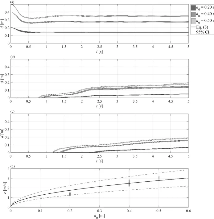
The hydrodynamic forcing condition was a dam-break wave, generated by the rapid release of a volume of water impounded behind a manually-opened swinging gate. Figure 3(a) – (c) shows the water surface elevations at x = - 0.10 m, 2.00 m, and 3.20 m for each impounded water depth (ℎ0 = 0.20 m, 0.40 m, and 0.50 m). For a full hydrodynamic analysis of the University of Ottawa Dam-break Flume, see Stolle et al. (2018b). The wave profiles were repeatable between experimental trials with a standard deviation in wave arrival time of 0.053 s and a standard deviation of the water surface of 0.008 m at the debris site (x = 3.20 m).
Figure 3. Time history of mean surface water elevation of the dam-break waves. The mean water surface elevations are provided for each impoundment at (a) WG1 (x = -0.10 m), (b) WG2 (x = 2.00 m), and (c) WG3 (x = 3.20 m). The wave front velocity (c) between WG2 and WG3 for each trial are shown in (d). The wave front velocity was fit to Eq. (4) (solid line), the 95% confidence interval of the fit is shown as the dashed line.
Due to challenges in measuring the flow velocity around the debris, the wave front velocity (𝑐𝑐) was used as a proxy for the local flow velocity. The wave front velocity was calculated by the difference in the wave arrival time between WG2 and WG3. Figure 3(d) shows the measured wave front velocity plotted against the impoundment depth. The wave front velocity is a function of the impoundment depth, flow resistance, and distance from the gate (Chanson 2006). Therefore, the velocity represents the mean velocity from x = 2.00 m and 3.20 m, and due to flow resistance across the area of interest, the wave front velocity will decrease. Eq. (4) is commonly used to describe the mean wave front velocity (Wüthrich et al. 2018)
𝑐𝑐 = 𝛼𝛼�𝑔𝑔ℎ0 (4)
where 𝛼𝛼 is a fitted coefficient. Literature values for the 𝛼𝛼-value can range from 0.66 (Matsutomi and Okamoto 2010) to 2.00 (Ritter 1892). Figure 3(d) shows the fitted Eq. (4), along with the 95% Confidence Interval (CI), for the mean wave velocity at the debris site resulting in 𝛼𝛼 = 1.29. Stolle et al. (2018b) performed a similar analysis for the debris length of the propagation section resulting in a fitted 𝛼𝛼-value of 1.09. Due to the relatively high flow resistance (f = 0.0293), the wave front velocity (and therefore 𝛼𝛼) decays rapidly across the area of interest.
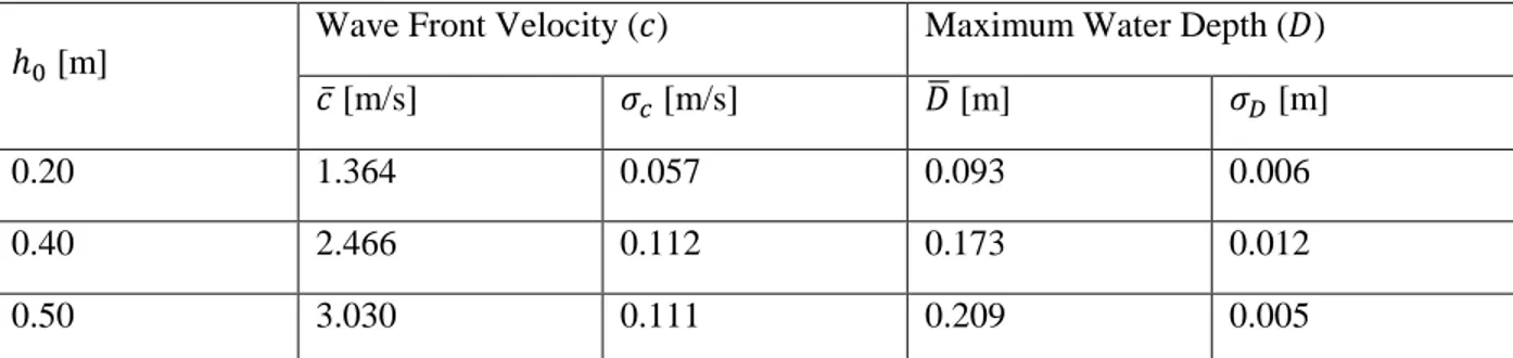
As the wave front velocity decays as it propagates downstream (Chanson 2006), the maximum drag forces acting on the debris occurred at the debris site. Therefore, for the remaining analysis, the wave front velocity will be used as the proxy for the local flow velocity. Due to the rapid nature of the debris entrainment and similar challenges measuring the local water depth, the maximum water depth (𝐷𝐷) at the debris site attained during single experimental runs was used for the following analysis. Table 2 outlines the mean (𝑐𝑐̅ and 𝐷𝐷�) and standard deviation (𝜎𝜎) for the wave front velocity and maximum water depth at the debris site for each impoundment depth. The data confirms the general trend of higher front velocities as well as increasing maximum water depth at the debris site with increasing impoundment reservoir depth. Low levels of standard deviation indicate the high degree of repeatability throughout the experimental campaign.
Table 2. Wave hydrodynamics at the debris site (x = 3.20 m).
ℎ0 [m]
Wave Front Velocity (𝑐𝑐) Maximum Water Depth (𝐷𝐷)
𝑐𝑐̅ [m/s] 𝜎𝜎𝑐𝑐 [m/s] 𝐷𝐷� [m] 𝜎𝜎𝐷𝐷 [m]
0.20 1.364 0.057 0.093 0.006
0.40 2.466 0.112 0.173 0.012
0.50 3.030 0.111 0.209 0.005
From a design perspective, information about the hydrodynamics driving the debris entrainment and consecutive downstream propagation is very important for the derivation of a probabilistic debris impact assessment. In the following, the path of the debris –its trajectory- will be discussed and evaluated for the given hydrodynamic conditions in the experiments.
3.3 Debris Trajectory
Assessing the likelihood of “extraordinary” debris impact has predominantly been performed in a binary manner (impact or no impact) due to challenges in identifying what parameter influence the trajectory of the debris. This section addresses the lateral (cross-flow) displacement (𝑌𝑌 = ∆𝑦𝑦/𝐷𝐷) of the debris, while the following section will address the displacement in the flow direction through assessing the debris velocity. The parameters addressed in this study were based on analysis of previous literature and the dimensional analysis performed in Section 3.1. As discussed in Section 2.3, the displacement was taken as the displacement from the geometric center of the initial configuration of debris.
In the framework develop by Lin and Vanmarcke (2010), the distribution of the debris trajectory was assumed to be a normal distribution with a mean of 0 (i.e., the debris propagates in a straight line). Stolle et al. (2018c) validated this assumption for a single shipping container in a similar experimental setup. As this study has used more than one piece of debris, they were assumed to act as a group spreading away from the debris source. Table 3 shows the mean (𝑌𝑌�) and standard deviation (𝜎𝜎𝑌𝑌) of the lateral displacement of the group of debris across the area of interest for each experimental category. A one-sample t-test (Anderson et al. 1958) was performed with the null hypothesis that the mean of the lateral displacement was equal to zero; the statistical test outcome is presented in Table 3. The data
predominantly confirms that the assumption of a mean of zero (p > 0.05) proofs to be correct except in the two cases with a single debris and an impoundment depth of 0.40 m. In addition, Stolle et al. (2018c) investigated similar test series and determined that the deviation from the mean was sufficiently small (less than the width of the shipping container). The remaining discrepancy was likely due to small inconsistencies in the bed topography.
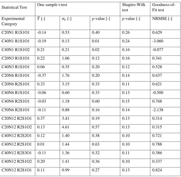
Table 3. Statistical properties of debris trajectories for each experimental category. The mean and standard deviation of lateral displacement are determined from the normalized lateral displacement (Y=∆y/D).
Statistical Test One sample t-test Shapiro-Wilk
test
Goodness-of-Fit test Experimental
Category
𝑌𝑌� [-] 𝜎𝜎𝑌𝑌 [-] p-value [-] p-value [-] NRMSE [-]
C20N1 R1S1O1 -0.14 0.53 0.40 0.26 0.629 C40N1 R1S1O1 -0.19 0.13 0.01 0.24 -3.060 C40N1 R1S1O2 0.21 0.21 0.02 0.16 -0.077 C20N3 R1S1O1 0.22 1.06 0.12 0.16 0.341 C40N3 R1S1O1 0.06 0.35 0.20 0.12 0.528 C20N6 R1S1O1 -0.37 1.76 0.20 0.14 0.637 C20N6 R2S1O1 0.33 3.15 0.33 0.11 0.621 C40N6 R1S1O1 -0.06 0.60 0.33 0.13 -0.500 C40N6 R2S1O1 -0.03 1.18 0.60 0.15 0.768 C50N6 R2S1O1 -0.11 0.88 0.16 0.14 -2.138 C20N12 R2S1O1 0.37 3.41 0.19 0.13 0.314 C20N12 R2S1O2 0.13 4.61 0.57 0.13 0.315 C40N12 R2S2O1 0.12 1.40 0.38 0.10 0.721 C40N12 R2S1O1 0.01 1.44 0.63 0.10 0.788 C40N12 R2S3O1 -0.11 1.36 0.32 0.11 0.386 C40N12 R2S1O2 0.20 1.41 0.36 0.10 0.337 C50N12 R2S1O1 0.11 0.99 0.27 0.13 0.824
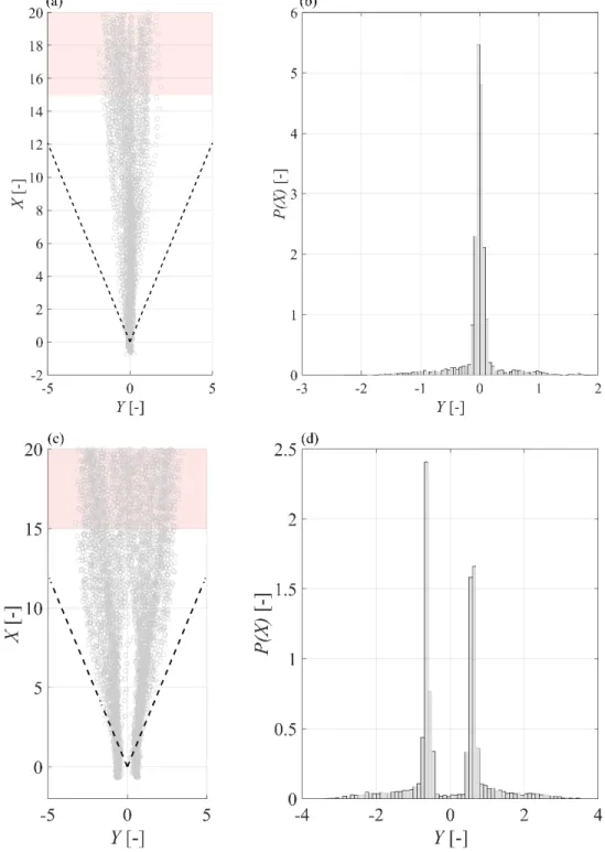
The second assumption made in Lin and Vanmarcke (2010) was the lateral displacement of the debris was normally distributed. Figure 4(a/c) shows the trajectories of debris for two experimental categories: C40N6 R1S1O1 and C40N12 R2S1O1. Each data point in the figure represents a measurement of a debris position obtained using the camera-based tracking algorithm. Figure 4(b/d) shows the probability density of the lateral displacements of debris over the whole area of interest. To test the assumption of normally distributed lateral displacements, a Shapiro-Wilk (1965) test was performed – with a significance of 95%
(𝛼𝛼 = 0.05) – with the null hypothesis that the lateral displacement was normally distributed around the mean. For each test, the p-value was reported in Table 3. If the p-value was less than 𝛼𝛼, the null hypothesis would be rejected (i.e. the lateral displacement of the debris could not be assumed to be normally distributed).
Figure 4. Debris transport for experimental category C40N6 R1S1O1 and C40N12 R2S1O1. (a, c) The position of each debris throughout the area of interest compared to the +/- 22.5o spreading angle suggested in Naito et al. (2014). The faded red box shows where the Shapiro-Wilk (1965) test was performed (in the final ∆X = 5). (b, d) Probability density of the lateral displacement throughout the area of interest.
For the cases with a single column of debris, the lateral displacement is normally distributed about the mean throughout the trajectory (Figure 4(a)). However, for the cases with two columns, this was not observed (p << 0.05) (Figure 4(c)). Due to the configuration of the debris, the lateral displacement (throughout the whole area of interest) has a distinct bimodal distribution (Figure 4(d)). As the debris continues to propagate from the debris site, the bimodality of the displacement decreased.
As the bimodality of the distribution introduced through the initial arrangement of debris began to diminish in the far-field and to simplify the distribution of the lateral displacements, the Shapiro-Wilk (1965) test was performed over the final ∆𝑋𝑋 = 5 (faded red box in Figure 4 – arbitrarily selected to represent the distribution of the debris in the far-field) of the area of interest. This adjustment was performed to reduce the influence of the initial configuration on the distribution – which will be captured in the estimation of the extents (through the standard deviation) as opposed to the shape of the distribution. As it can be seen from Table 3, in the latter stages of the propagation, all experimental categories displayed normally distributed lateral displacement about the mean (p > 0.05).
Based on the assumption of a normal distribution with a mean displacement of the debris group equal to zero, the probability density function (𝑃𝑃) can be expressed as:
𝑃𝑃(𝑋𝑋) = 1 �2𝜋𝜋𝜎𝜎𝑌𝑌2
𝑅𝑅− 𝑌𝑌
2
2𝜎𝜎𝑌𝑌2 (5)
Therefore, the only free parameter is the standard deviation. While the Shapiro-Wilk (1965) test showed that the initial configuration did not influence the shape of the distribution of the debris in the latter stages of the flow, it did influence the standard deviation. To address the various parameters outlined in the dimensional analysis, multiple linear regression was performed to examine the influence of the outlined parameters on the standard deviation. The standard deviation was determined as a function of the displacement (𝑋𝑋) from the debris source for each experimental category.
The variance inflation factor (VIF) (Kenney 1962) was calculated between each of the parameters outlined in Section 3.1 to test for multicollinearity between the parameters. Multicollinearity can result in large fluctuations in estimated coefficients from the regression. Generally, VIF values greater than 10 indicate collinearity between variables (Farrar and Glauber 1967). In this case, 𝐹𝐹𝑟𝑟 and 𝑅𝑅𝑅𝑅 exhibited, as they both characterize the hydrodynamics, high collinearity (VIF > 10). This collinearity between 𝐹𝐹𝑟𝑟 and 𝑅𝑅𝑅𝑅 does not always hold for the case of a tsunami wave. Instead, this collinearity is related to representing the initial inundation as a break wave (Chanson 2006), it is expected due to the physics of the dam-break problem – the faster flow occurs in the wave tip (the region characterized by the shallower water depth) and then it slows down in the subsequent wave body (characterized by deeper water conditions). Furthermore, while the model was scaled using the Froude similitude criterion, the Reynolds number from the experiment does not represent ranges that are typical of tsunami. Therefore, the Reynolds number was not considered in the regression analysis, but it should be considered in future studies addressing different stages of the tsunami inundation. The ratio 𝑙𝑙/𝐷𝐷 and parameter Θ also displayed high VIF values, as the parameter Θ was related to the orientation of the long axis. The parameter Θ was hence removed from the analysis (and was not included in Table 4) as it does not represent a physical characteristic in the force balance and the length of exposed area to the flow (𝑙𝑙 or characteristic length) is commonly used to represent the projected area of an object in the estimation of drag forces. As the remaining factors are a function of the initial configuration, these parameters are assumed to influence the change in standard deviation over distance from the site, resulting in the equation:
𝜎𝜎𝑌𝑌= ��𝜆𝜆1Fr+ 𝜆𝜆2𝐷𝐷 + 𝜆𝜆𝑙𝑙 3𝐷𝐷 + 𝜆𝜆𝑆𝑆 4𝑛𝑛 + 𝜆𝜆5𝑟𝑟� 𝑋𝑋 + 𝑋𝑋𝑖𝑖� (6)
where 𝜆𝜆𝑗𝑗 are the regression coefficients (with j the numbers of coefficients) and 𝑋𝑋𝑖𝑖 is the position of the outermost columns of debris in the initial configuration (Figure 1).
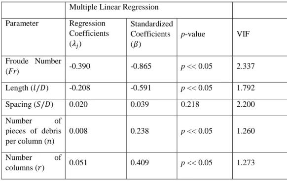
Table 4. Multiple linear regression of the standard deviation of the debris displacement (Y).
Multiple Linear Regression
Parameter Regression Coefficients (𝜆𝜆𝑗𝑗) Standardized Coefficients (𝛽𝛽) p-value VIF Froude Number (Fr) -0.390 -0.865 p << 0.05 2.337 Length (𝑙𝑙/𝐷𝐷) -0.208 -0.591 p << 0.05 1.792 Spacing (𝑆𝑆/𝐷𝐷) 0.020 0.039 0.218 2.200 Number of pieces of debris per column (𝑛𝑛) 0.008 0.238 p << 0.05 1.260 Number of columns (𝑟𝑟) 0.051 0.409 p << 0.05 1.273
The multiple linear regression showed that the linearized model could explain 62% of the margin of variance (R2 = 0.617) and was statistically significant (p << 0.05). A Kolmogrov-Smirnov test (Smirnov 1948) was performed with the null hypothesis that the residual were normally distributed, ensuring the validation of the assumption of normally distributed residuals (p = 0.10). Each of the coefficients was considered to show a statistically significant trend, except in the case of spacing. This is potentially due to the limited number of cases that examined the influence of spacing as well as a high potential for a non-linearity that cannot be captured by the regression model. Rueben et al. (2014) noted, in a study of debris dynamics over a slope surface, that the debris appeared to have an “area of influence” related to their obstruction of the flow. Similar to a fixed obstacle, debris influence the surrounding flow as they tend to propagate slower than the surrounding fluid. Therefore, it is likely that the area of influence is a function of the inertia of the debris, hydrodynamics, and spacing. Further investigation is necessary to address the importance of spacing within this context.
The calculated regression coefficients (shown in Table 4) are subject to potential scale effects and are influenced by parameters not included within the regression, such as friction and buoyancy. However, the standardized coefficient, where the regression was performed with each standardized parameter (i.e., mean of 0 and standard deviation of 1), show the relative influence of each parameter on the lateral displacement.
Based on the standardized coefficients (Table 4), the hydrodynamic conditions, the exposed length of the debris, and the number of columns have the most substantial influence on the lateral displacement. This is consistent with previous literature, Stolle et al. (2018c) which indicated that, for a single debris, the greater water depths and velocities resulted in smaller lateral displacement due to less interaction with bed surface. Braudrick and Grant (2001) determined that the debris tended towards a equilibrium orientation, in the case of shipping containers with the long axis perpendicular to the flow, during the rotation process this causes an increase in the lateral displacement. Stolle et al. (2018d) showed that the debris tended to diffuse away from the initial configuration as a function of the number of columns present. Nistor et al. (2016) showed that the increase in the number of pieces of debris resulted in an increase in the lateral displacement.
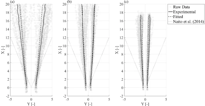
The fit of Eq. (6) to each experimental category was estimated using the normalized root mean squared error (NRMSE): 𝑁𝑁𝑅𝑅𝑁𝑁𝑆𝑆𝑁𝑁 = 1 −∑ �𝜎𝜎𝑌𝑌�𝑋𝑋𝑗𝑗� − 𝜎𝜎��𝑋𝑋𝑌𝑌 𝑗𝑗�� 𝑚𝑚 𝑗𝑗=1 ∑ �𝜎𝜎𝑚𝑚𝑗𝑗=1 𝑌𝑌�𝑋𝑋𝑗𝑗� − 𝜎𝜎����𝑌𝑌 (7) where 𝜎𝜎𝑌𝑌 is the standard deviation from the experimental data, 𝜎𝜎� is the standard deviation estimated 𝑌𝑌 from Eq. (6), 𝜎𝜎��� is the mean standard deviation, and 𝑚𝑚 is the number of data points. The NRMSE can 𝑌𝑌 range from 1 (perfect fit) to -∞ (bad fit). The NRMSE for each experimental category is shown in Table 3. Figure 5 shows a comparison of the fit for three identical debris configurations with different hydrodynamic forcing conditions with NRMSE equal to 0.621 (a), 0.768 (b), and -2.138 (c), respectively. Eq. (6) had difficulty modelling small changes in standard deviation over area of interest (i.e. Figure 5(c)), though overall modelled each experimental category well.
Figure 5. Comparison of the fitted standard deviation (dashed line), standard deviation from the experimental data (solid line), and the raw experimental data (circular markers) for experimental categories with 6 debris, 2 columns, 0.03 m spacing, and 0o orientation: (a) C20N6 R2S1O1; (b) C40N6 R2S1O1; and (c) C50N6 R2S1O1.
3.4 Debris Velocity
The debris velocity is a critical intermediate component of debris hazard assessment as it dictates the magnitude of the impact force exerted on the structure (Eq. (1), Nistor et al. (2017)). Stolle et al. (2017) examined the transport of multiple shipping containers in similar configurations as the ones investigated in this study. Based on a force balance of fully entrained debris, the following equation was determined to describe the debris velocity:
𝑢𝑢 = 𝑐𝑐 − �𝐶𝐶2𝑛𝑛𝑚𝑚𝑑𝑑𝜌𝜌𝑤𝑤𝐴𝐴𝑑𝑑 𝑑𝑑 𝑡𝑡 + 1 𝑐𝑐� −1 (8) where 𝐶𝐶𝑑𝑑 is the drag coefficient of the debris and 𝐴𝐴𝑑𝑑 is the cross-sectional area of the debris exposed to the flow. Eq. (8) does not consider the entrainment of the debris, which requires further development due to the different potential modes of transport (i.e. sliding, rotation). Furthermore, as the local flow velocity around the debris is a difficult parameter to estimated, the wave front velocity is used as a proxy for the
flow velocity. Eq. (8) represents a conservative estimation of the debris velocity over a flat horizontal surface as the wave front velocity will represent the maximum flow velocity.
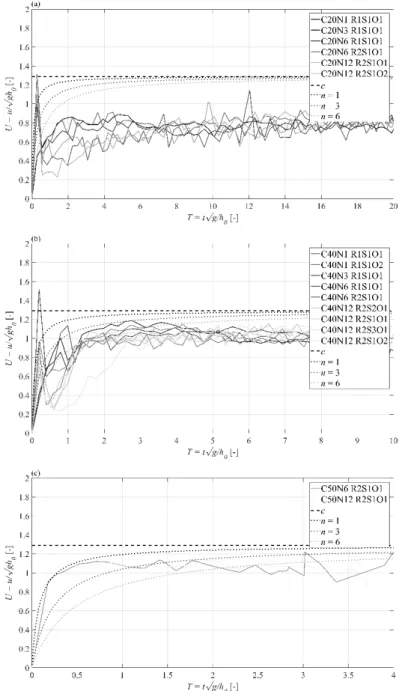
Figure 6 shows the mean group velocity of the debris for each of the experimental categories as a function of time, separated by the initial impoundment depth. Eq. (8), based on the number of pieces of debris present within each column, is shown as a dotted line. As it can be seen from Eq. (8), the debris velocity approaches the wave front velocity asymptotically. Comparing the debris velocity to the mean wave front velocity at the site (Eq. (4), 𝛼𝛼 = 1.29), the debris group velocity does not exceed the wave front velocity, as expected. As the wave front velocity decays over the area of interest, the debris does not reach the wave front velocity at the debris site and instead approaches the mean wave front velocity over the area of interest (𝛼𝛼 = 1.09), as determined from Stolle et al. (2018b).
Figure 6. Mean debris velocity (solid lines) for each experimental category for (a) h0 = 0.20 m, (b) h0 = 0.40 m, and (c) h0 =
0.50 m. The dotted line shows the estimated velocity from Eq. (8). The thick dashed line details the mean wave front velocity based on Eq. (4).
The rapid acceleration of the debris in the initial phases of entrainment is not captured by Eq. (8). As described in Stolle et al. (2015), at smaller impoundment depths, the initial wave impact does not initiate the motion of the debris. As a result, a wake forms downstream from the debris, causing a large hydraulic gradient between the upstream and downstream faces of the debris. Once the horizontal force induced by the hydraulic gradient overcomes the static friction force, the debris rapidly accelerates, in some cases, briefly exceeding the wave front velocity. However, as the debris settles within the wave front, the debris velocity reduces to below the wave front velocity. In the case of ℎ0 = 0.50 m, the momentum of the wave immediately overcomes the coefficient of static friction, resulting in no rapid spike in the acceleration of the debris.
While Eq. (8) does not capture the entrainment phase of debris transport, the equation does represent a conservative estimation (with 𝑛𝑛 = 1) of the evolution of the mean velocity over time. To capture the probabilistic nature of debris transport, Lin and Vanmarcke (2010) suggested the application of a bounded distribution to capture the evolution of debris velocity between rest and the maximum flow velocity. Lin and Vanmarcke (2010) used a Beta distribution (McDonald 2009), however, the challenge with the Beta distribution is that the distribution requires a specialized Beta function to ensure that the total probability remains constant. The Kumaraswamy (1980) (K1980) two-parameter (𝑎𝑎 and 𝑏𝑏) bounded distribution, developed for hydrology application (Jones 2009), is within the same family as the Beta distribution. The K1980 distribution represents a similarly shaped distribution with the distinct advantage of having a closed form for both the probability (𝑓𝑓(𝑥𝑥; 𝑎𝑎, 𝑏𝑏)) and cumulative distribution (𝐹𝐹(𝑥𝑥; 𝑎𝑎, 𝑏𝑏)) functions:
𝑓𝑓(𝑈𝑈; 𝑎𝑎, 𝑏𝑏) = 𝑎𝑎𝑏𝑏𝑈𝑈𝑎𝑎−1(1 − 𝑈𝑈𝑎𝑎)𝑏𝑏−1 (9)
𝐹𝐹(𝑥𝑥; 𝑎𝑎, 𝑏𝑏) = 1 − (1 − 𝑈𝑈𝑎𝑎)𝑏𝑏 (10)
Similar to the Beta distribution, the K1980 distribution is determined by its mean (𝑈𝑈�) and dispersion (𝜂𝜂𝑈𝑈), expressed in the shape terms as:
𝑎𝑎 = 𝑈𝑈�𝜂𝜂𝑢𝑢 (11)
𝑏𝑏 = (1 − 𝑈𝑈�)𝜂𝜂𝑢𝑢 (12)
Using Eq. (8), the normalized debris velocity can be determined as: 𝑈𝑈� =𝑢𝑢 𝑐𝑐 = 1 − � 𝐶𝐶𝑑𝑑𝜌𝜌𝑤𝑤𝐴𝐴𝑑𝑑 2𝑛𝑛𝑚𝑚𝑑𝑑 𝑐𝑐𝑡𝑡 + 1� −1 (13) The K1980 distribution can take on different shapes depending on 𝑎𝑎 and 𝑏𝑏, however, for the purpose of debris transport, the distribution should be unimodal (Lin and Vanmarcke 2010). Therefore, the values of 𝑎𝑎 and 𝑏𝑏, must be greater than 1.0 (Jones 2009). Based on Eq. (11) and (12), the dispersion must then be defined as:
𝜂𝜂𝑢𝑢 = max �𝑈𝑈�1,1 − 𝑈𝑈�1 � + 𝛾𝛾 (14)
where 𝛾𝛾 is a positive fitted parameter based on the type of debris. Using the experimental data, the parameter 𝛾𝛾 was iteratively fit to the data set (𝛾𝛾 = 2.32) by comparing the mean squared errors between the experimental and theoretical probability density functions (PDF). The applicability of the K1980 distribution was then evaluated using the Kolmogorov-Smirnov test, which compares the experimental cumulative distribution function (CDF) to the theoretical one (Smirnov 1948), with the null hypothesis that the experimental data follows the K1980 distribution at each time step.
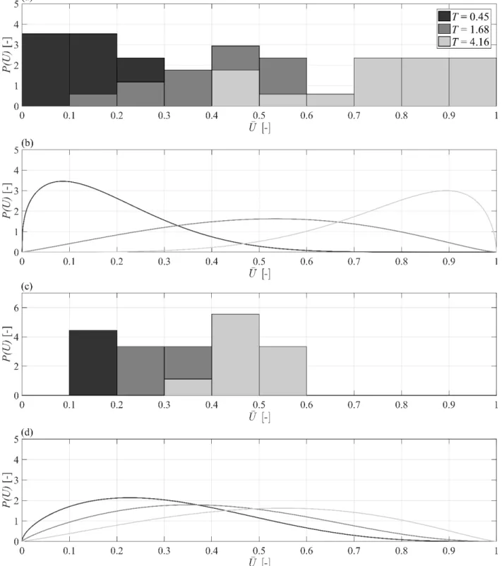
For each experimental category, the null hypothesis was not rejected with a mean p-value of 0.30 (+/- 0.09). Therefore, the K1980 distribution can be assumed to reasonably capture the experimental dataset. Figure 7 shows a comparison of the experimental data set ((a) and (c)) to the proposed K1980 distribution ((b) and (d)) for two experimental categories (C40N1 R1S1O1 and C40N12 R2S1O1, respectively) at three arbitrarily selected time steps. As the time passes, the mean velocity of the debris increased towards the wave front velocity in both experimental cases. However, the influence of the added inertia in the case
with 12 debris (Figure 7(c)) can be observed by the reduced velocity in the later time steps compared to the single debris case.
Figure 7. Comparison of the probability density function (P(U)) for the experimental data set (a, c) to the theoretical Kumaraswamy (1980) distribution (b, d) for three time steps for C40N1 R1S1O1 and C40N12 R2S1O1, respectively.
4
Application
Although the proposed model has some limitations due to scale and model effects (discussed in following section), the framework introduced in this work is intended to provide insight into the necessary effects (through physically-meaningful parameters) to be addressed when assessing debris hazard in tsunami-like flow events. To illustrate the application of this framework to an engineering problem, a simplified example is presented in this section. The debris investigated in this example will be empty shipping containers (6.10 m × 2.40 m × 2.40 m, mass = 2 270 kg, stiffness (𝑘𝑘) = 42 900 kN/m) (ASCE 2016). The debris source is assumed to be located 50 m from the critical structure’s design site (∆𝑥𝑥). The debris configuration consists of 6 debris (𝑛𝑛) set in a single column (𝑟𝑟) with the long axis perpendicular to the flow direction (Figure 8). The direction of the flow is assumed to be directly normal the average shoreline, similar to the assumption provided by the ASCE7 Chapter 6. The centroid of the design site is 20 m from the normal (∆𝑦𝑦). The width of the design site (𝑤𝑤) is 20 m. The water depth and flow velocity at the debris source would normally need to be determined through modelling or the energy grade line (Kriebel et al. 2017) presented in the ASCE7 Chapter 6. For this exercise, the flow velocity and water depth were assumed to be 6 m/s and 4 m, respectively. Using the method proposed above, the objective is to calculate the probability of debris impact occurring and magnitude of the impact force (through the impact velocity, Eq. (1)).
Figure 8. Engineering application of probabilistic model for debris hazard analysis. The initial configuration the debris is shown in the sub-figure.
In determining the impact velocity, the time for the debris to reach the design site must be determined. Integrating Eq. (8) results in the following equation for debris displacement:
∆𝑥𝑥 = 𝑐𝑐𝑡𝑡 −𝐶𝐶2𝑛𝑛𝑚𝑚𝑑𝑑
𝑑𝑑𝜌𝜌𝑤𝑤𝐴𝐴𝑑𝑑ln �
𝐶𝐶𝑑𝑑𝜌𝜌𝑤𝑤𝐴𝐴𝑑𝑑
2𝑚𝑚𝑑𝑑 𝑐𝑐𝑡𝑡 + 1�
(15) Solving for 𝑡𝑡 and 𝑈𝑈 (using Eq. (8)) results in values of 9.36 s and 5.81 m/s, respectively (Figure 9(a)). Using the mean velocity, the shape parameters for the probability density function (Eq. (9)) (𝑎𝑎 and 𝑏𝑏) can be calculated using Eq. (11) and (12). Using Eq. (10), the likelihood of the impact velocity being less than a value could be determined, however, the complement of that probability (1 − 𝐹𝐹(𝑈𝑈; 𝑎𝑎, 𝑏𝑏)) is the likelihood an impact velocity will exceed a certain value, which is a more useful value for practicing engineers. Applying Eq. (1), the likelihood of exceedance of a certain impact force can be determined (Figure 9(c)).
Figure 9. Figure 9. Calculation of (a) mean impact velocity (Eq. (8)), (b) probability density function of the impact velocity (Eq. (9)); and (c) survival function for the design impact force (Eq. (10)).
As discussed in Section 3.3, the mean lateral displacement of the debris will be assumed to be 0. The standard deviation can be calculated using Eq. (6), resulting in a value of 7.40. The probability density function can then be calculated for a distance of 50 m from the debris source (Figure 10). It is assumed that debris will only make contact with the front face of the structure. Integrating the probability density function across the face of the structure (red faded box in Figure 10), the resulting probability of impact is approximately 21%.
Figure 10. Calculation of the probability of impact based on Eq. (5). The faded red box shows the location of the design site.
5
Discussion
The experimental setup was intended to represent an idealized case of a tsunami propagating over coastal plain (Chanson 2006). To ensure the experiment could adequately address the probabilistic nature of debris transport, the scope was limited to represent this specific scenario. As such, the hydrodynamic boundary condition only examined the initial inundation of a broken tsunami wave and did not consider the results of drawdown or subsequent wave entrainment. The number of pieces of debris was limited to a maximum of 12 as further additions resulted in significant model effects due to interactions with the walls of the flume. The inter-debris friction, debris-bed friction, and the buoyancy of the debris were not investigated. Additionally, only a single geometry was investigated (a cuboid), although the characteristic length was included in Eq. (6) to potentially consider other geometries in future works. As these factors have been shown to have an influence on debris transport, further research is necessary to address these issues.
Bricker et al. (2015), in a study examining Manning’s roughness coefficients used in tsunami modelling, indicated the critical importance in adequately addressing viscous and surface tension effects. Within the present experiment, the Reynolds number ranged from 1.59 × 10⁴ to 6.85 × 10⁵ which places the flow within the turbulent flow regime (Te Chow 1959). However, as the Reynolds number at prototype scale are often in excess of 1.00 × 10⁶ – as such, the experiments presented herein do not fully capture the turbulent boundary layer’s dynamics (Sumer and Fredsøe 2006), influencing the drag forces on the debris. The Weber number (𝑊𝑊𝑅𝑅 = 𝜌𝜌𝑈𝑈2𝐷𝐷/𝜎𝜎), the ratio of surface tension and gravitational forces, ranged from 152.4 to 671.2 exceeding the critical Weber number of 120 prescribed by Peakall and Warburton (1996). However, concerns potentially exist between the debris where adhesion may occur.
For the lateral displacement of the debris, it would be expected that the general importance and influence of the parameters discussed in Sections 3.1 and 3.3 would remain similar at prototype scale. However, the magnitude of regression coefficients (𝜆𝜆𝑗𝑗) could potentially vary significantly. To date, no study has investigated debris motion at sufficiently large scales to address scale effects while this work depicts the first approach towards describing the debris transport process probabilistically where extreme flow conditions are concerned. In particular, parameters, such as turbulence (She and Leveque 1994) and drag (Granville 1976), which scale considering Reynolds similitude are not properly scaled. Additionally, this study did not address parameters that would have a significant influence on debris transport, in particular, buoyancy and friction. As shown in Section 3.3, the Eq. (6) could not describe 38% of the variance from the mean, leaving potential to build upon the current data set to address these issues.
The evolution of the debris velocity should theoretically be more robust to scale effects as the underlying Eq. (8) is based on a closed solution of the forces acting on the debris. However, as discussed in Section 3.4, the equation was based on fully entrained debris, and therefore, does not consider the influence of debris entrainment or other forms of motion, such as sliding or saltation. Though, as these phases of
motion would result in loss of energy and, therefore, reduced acceleration, Eq. (8) represents a conservative estimation of the potential debris velocity at a given time.
The experimental study presented here examined the transport of “extraordinary” debris in a dam-break wave over a flat, horizontal surface. Therefore, certain limitations need to be addressed in the application of the model in a built environment. Several aspects, such as flow channelling or typical surface roughness of debris, are not captured with the current model. Investigation is also necessary to address debris transport through flow obstructions (Goseberg et al. 2016), likely influencing the underlying assumption that the mean displacement of the debris is equal to zero. Additionally, this study only considered a single distribution to represent the lateral displacement; further work could incorporate studies of skew and kurtosis to address potential limitations of not considering the third and fourth moments of the statistical distribution.
Flow accelerations and impact with other structures within these constricted environments may influence the evolution of the debris velocity. Furthermore, the model examines “extraordinary” debris impact where the debris has a distinct source and is immediately entrained within the flow. Other probabilistic models have also included terms that consider debris generation (i.e., from the destruction of houses), the generation of individual debris objects is then modelled as a Poisson distribution (Lin and Vanmarcke 2010, Hatzikyriakou and Lin 2017). However, as the accurate modelling of collapsing structures under hydraulic loading has yet to be addressed, this aspect was not included within this study (Heller 2011).
6
Conclusions
The experiments presented here were used in the development of a probabilistic framework for addressing debris hazard in extreme flooding events. Using the measured trajectory of debris within energetic flow events and dimensional analysis, empirical formulas were developed capturing the physical motion in a probabilistic framework. Based on the results of these experiments the following conclusions can be derived:
• The mean trajectory of the debris group (from the center of the debris source) over a horizontal surface, with no flow obstruction, can be estimated with no lateral displacement. The distribution of lateral displacement around the mean can be assumed to be Gaussian.
• The hydrodynamic conditions, geometry of the debris, as well as the initial arrangement configuration of the debris were determined to be the most important factors (in that order) influencing the lateral distribution of the debris entrained within the flow.
• A force balance of completely entrained debris can be used to conservatively estimate the evolution of debris velocity as a function of time.
• The distribution of debris velocity as a function of time can be estimated using a two-parameter bounded distribution, the Kumaraswamy (1980) distribution.
The proposed model was developed analyzing the general trends regarding debris motion, in particular, their lateral motion. However, potential scale effects need to be addressed before the application of such a model. With the challenges in assessing debris trajectory in the aftermath of events through field studies, future investigations into debris hazard assessment will need to be conducted at sufficiently large scale to limit scale effects related to the Reynolds number, in particular, turbulence and drag. The results discussed herein should aid in the development of such experimental series as it helps inform general parameters that are critical in the assessment of debris displacement.
Data Availability Statement
Some or all data, models, or code that support the findings of this study are available from the corresponding author upon reasonable request including: raw data from hydraulic measurements and video footage as well as Matlab code for analysis methods.
Acknowledgements
The authors would like to acknowledge the support of the NSERC CGS-D Scholarship (Jacob Stolle), of the NSERC Discovery Grant [No. 210282] (Ioan Nistor) and of the Marie Curie International Outgoing Fellowship within the 7th European Community Framework Program [No. 622214] (Nils Goseberg).
References
Anderson, T. W., T. W. Anderson, T. W. Anderson, T. W. Anderson, and E.-U. Mathématicien. 1958. An introduction to multivariate statistical analysis. . Wiley New York.
ASCE. 2016. Minimum design loads for buildings and other structures. . American Society of Civil Engineers.
Braudrick, C. A., and G. E. Grant. 2000. When do logs move in rivers? Water resources research 36:571– 583.
Braudrick, C. A., and G. E. Grant. 2001. Transport and deposition of large woody debris in streams: a flume experiment. Geomorphology 41:263–283.
Bricker, J. D., S. Gibson, H. Takagi, and F. Imamura. 2015. On the need for larger Manning’s roughness coefficients in depth-integrated tsunami inundation models. Coastal Engineering Journal 57:1550005.
Chanson, H. 2006. Tsunami surges on dry coastal plains: Application of dam break wave equations. Coastal Engineering Journal 48:355–370.
Charvet, I., A. Suppasri, H. Kimura, D. Sugawara, and F. Imamura. 2015. A multivariate generalized linear tsunami fragility model for Kesennuma City based on maximum flow depths, velocities and debris impact, with evaluation of predictive accuracy. Natural Hazards 79:2073–2099.
Chock, G. Y. 2016. Design for tsunami loads and effects in the ASCE 7-16 standard. Journal of Structural Engineering:04016093.
Derschum, C., I. Nistor, J. Stolle, and N. Goseberg. 2018. Debris impact under extreme hydrodynamic conditions part 1: Hydrodynamics and impact geometry. Coastal Engineering.
Farrar, D. E., and R. R. Glauber. 1967. Multicollinearity in regression analysis: the problem revisited. The Review of Economic and Statistics:92–107.
GDV. 2003. Cargo loss prevention information from German marine insurers. Container Handbook. Goseberg, N., J. Stolle, I. Nistor, and T. Shibayama. 2016. Experimental analysis of debris motion due the
obstruction from fixed obstacles in tsunami-like flow conditions. Coastal Engineering 118:35–49. Granville, P. S. 1976. Elements of the drag of underwater bodies. . DTIC Document.
Haehnel, R. B., and S. F. Daly. 2004. Maximum impact force of woody debris on floodplain structures. Journal of Hydraulic Engineering 130:112–120.
Häfen, H. von, J. Stolle, N. Goseberg, and I. Nistor. 2018. Lift and Swing Gate Modelling For Dam-break Generation With A Particle-Based Method.
Hatzikyriakou, A., and N. Lin. 2017. Impact of performance interdependencies on structural vulnerability: A systems perspective of storm surge risk to coastal residential communities. Reliability Engineering & System Safety 158:106–116.
Heller, V. 2011. Scale effects in physical hydraulic engineering models. Journal of Hydraulic Research 49:293–306.
Hughes, S. A. 1993. Physical models and laboratory techniques in coastal engineering. . World Scientific. Jones, M. 2009. Kumaraswamy’s distribution: A beta-type distribution with some tractability advantages.
Statistical Methodology 6:70–81.
Kenney, J. F. 1962. Mathematics of Statistics. Pages 77–80 in E. S. Keeping, editor., 3rd edition. Van Nostrand, Princton, NJ.
Knorr, W., and F. Kutzner. 2008. EcoTransIT: Ecological Transport Information Tool - Environmental Method and Data. . IFEU Heidelberg.
Kriebel, D. L., P. J. Lynett, D. T. Cox, C. M. Petroff, I. N. Robertson, and G. Y. Chock. 2017. Energy method for approximating overland tsunami flows. Journal of Waterway, Port, Coastal, and Ocean Engineering 143:04017014.
Kumaraswamy, P. 1980. A generalized probability density function for double-bounded random processes. Journal of Hydrology 46:79–88.
Lin, N., and E. Vanmarcke. 2010. Windborne debris risk analysis—Part I. Introduction and methodology. Wind and Structures 13:191.
Macabuag, J., A. Raby, A. Pomonis, I. Nistor, S. Wilkinson, and T. Rossetto. 2018. Tsunami design procedures for engineered buildings: a critical review. Proceedings of the Institution of Civil Engineers: Civil Engineering. . Thomas Telford.
Matsutomi, H., and K. Okamoto. 2010. Inundation flow velocity of tsunami on land. Island Arc 19:443– 457.
McDonald, J. H. 2009. Handbook of biological statistics. . Sparky House Publishing Baltimore, MD. Mori, N., T. Takahashi, T. Yasuda, and H. Yanagisawa. 2011. Survey of 2011 Tohoku earthquake
tsunami inundation and run-up. Geophysical Research Letters 38.
Naito, C., C. Cercone, H. R. Riggs, and D. Cox. 2014. Procedure for site assessment of the potential for tsunami debris impact. Journal of Waterway, Port, Coastal and Ocean Engineering 140:223–232. Nistor, I., N. Goseberg, T. Mikami, T. Shibayama, J. Stolle, R. Nakamura, and S. Matsuba. 2016.
Hydraulic Experiments on Debris Dynamics over a Horizontal Plane. Journal of Waterway, Port, Coastal and Ocean Engineering:04016022.
Nistor, I., N. Goseberg, and J. Stolle. 2017. Tsunami-Driven Debris Motion and Loads: A Critical Review. Frontiers in Built Environment 3:2.
Peakall, J., and J. Warburton. 1996. Surface tension in small hydraulic river models-the significance of the Weber number. Journal of Hydrology New Zealand 35:199–212.
Reese, S., B. A. Bradley, J. Bind, G. Smart, W. Power, and J. Sturman. 2011. Empirical building fragilities from observed damage in the 2009 South Pacific tsunami. Earth-Science Reviews 107:156–173.
Ritter, A. 1892. Die fortpflanzung der wasserwellen. Zeitschrift Verein Deutscher Ingenieure 36:947–954. Rueben, M., D. Cox, R. Holman, S. Shin, and J. Stanley. 2014. Optical Measurements of Tsunami
Inundation and Debris Movement in a Large-Scale Wave Basin. Journal of Waterway, Port, Coastal, and Ocean Engineering 141.
Shafiei, S., B. W. Melville, A. Y. Shamseldin, S. Beskhyroun, and K. N. Adams. 2016. Measurements of tsunami-borne debris impact on structures using an embedded accelerometer. Journal of Hydraulic Research 54:1–15.
Shapiro, S. S., and M. B. Wilk. 1965. An analysis of variance test for normality (complete samples). Biometrika 52:591–611.
She, Z.-S., and E. Leveque. 1994. Universal scaling laws in fully developed turbulence. Physical review letters 72:336.
Smirnov, N. 1948. Table for estimating the goodness of fit of empirical distributions. The annals of mathematical statistics 19:279–281.
Stolle, J., C. Derschum, N. Goseberg, I. Nistor, and E. Petriu. 2018a. Debris impact under extreme hydrodynamic conditions part 2: Impact force responses for non-rigid debris collisions. Coastal Engineering 141:107–118.
Stolle, J., B. Ghodoosipour, C. Derschum, I. Nistor, E. Petriu, and N. Goseberg. 2018b. Swing Gate Generated Dam-break Waves. Journal of Hydraulic Research In-Press.
Stolle, J., N. Goseberg, I. Nistor, and E. Petriu. 2018c. Probabilistic Investigation and Risk Assessment of Debris Transport in Extreme Hydrodynamic Conditions. Journal of Waterways, Ports, Oceans and Coastal Engineering 144:04017039.
Stolle, J., N. Goseberg, I. Nistor, and E. Petriu. 2019. Debris Impact Forces on Flexible Structures in Extreme Hydrodynamic Conditions. Journal of Fluids and Structures Under Review.
Stolle, J., I. Nistor, and N. Goseberg. 2016. Optical Tracking of Floating Shipping Containers in a High-Velocity Flow. Coastal Engineering Journal 58:1650005.
Stolle, J., I. Nistor, N. Goseberg, T. Mikami, and T. Shibayama. 2017. Entrainment and Transport Dynamics of Shipping Containers in Extreme Hydrodynamic Conditions. Coastal Engineering Journal 59:1750011.
Stolle, J., I. Nistor, N. Goseberg, T. Mikami, T. Shibayama, R. Nakamura, and S. Matsuba. 2015. Flood-Induced Debris Dynamics over a Horizontal Surface. Coastal Structures and Solutions to Coastal Disasters. . ASCE-COPRI.
Stolle, J., T. Takabatake, G. Hamano, H. Ishii, K. Iimura, T. Shibayama, I. Nistor, N. Goseberg, and E. Petriu. 2018d. Debris Transport over a Sloped Surface in Tsunami-Like Flow Conditions. Coastal Engineering Journal Under Review.
Sumer, B. M., and J. Fredsøe. 2006. Hydrodynamics around cylindrical structures. . World Scientific. Te Chow, V. 1959. Open channel hydraulics. . McGraw-Hill Book Company, Inc; New York.
Wüthrich, D., M. Pfister, I. Nistor, and A. J. Schleiss. 2018. Experimental study on forces exerted on buildings with openings due to extreme hydrodynamic events. Coastal Engineering.