Atomistic simulation of fatigue in face centred cubic metals

(1)

HAL Id: tel-01526211

https://pastel.archives-ouvertes.fr/tel-01526211

Submitted on 22 May 2017

HAL is a multi-disciplinary open access archive for the deposit and dissemination of sci-entific research documents, whether they are pub-lished or not. The documents may come from teaching and research institutions in France or abroad, or from public or private research centers.

L’archive ouverte pluridisciplinaire HAL, est destinée au dépôt et à la diffusion de documents scientifiques de niveau recherche, publiés ou non, émanant des établissements d’enseignement et de recherche français ou étrangers, des laboratoires publics ou privés.

Atomistic simulation of fatigue in face centred cubic

metals

Zhengxuan Fan

To cite this version:

Zhengxuan Fan. Atomistic simulation of fatigue in face centred cubic metals. Mechanics of materials [physics.class-ph]. Université Paris Saclay (COmUE), 2016. English. �NNT : 2016SACLX076�. �tel-01526211�

(2)

i

NNT : 2016SACLX076

THÈSE DE DOCTORAT

DE L'UNIVERSITÉ PARIS-SACLAY

préparée à l'ÉCOLE POLYTECHNIQUE

ECOLE DOCTORALE N° 573

Interfaces — Approches interdisciplinaires : fondements, applications et innovations Spécialité :PHYSIQUE

par

Mme Zhengxuan FAN

Simulation atomistique de la fatigue dans les métaux

cubiques à faces centrées

Thèse soutenue à Palaiseau le 18 novembre 2016

Composition du jury :

Mme Sandrine BROCHARD Rapporteur M. Derek WARNER Rapporteur M. Gilbert HÉNAFF Président M. Haël MUGHRABI Examinateur M. Boubakar DIAWARA Examinateur M. Maxime SAUZAY Co-directeur M. Olivier HARDOUIN DUPARC Directeur

(3)

(4)

iii

NNT : 2016SACLX076

Thesis to be presented to obtain the degree of

DOCTOR OF UNIVERSITÉ PARIS-SACLAY

prepared at the ÉCOLE POLYTECHNIQUE

DOCTORAL SCHOOL No. 573

Interfaces — Approches interdisciplinaires : fondements, applications et innovations Speciality:PHYSICS

by

Zhengxuan FAN

Atomistic simulation of fatigue in face centred cubic

metals

Thesis defended at Palaiseau 18 November 2016

Thesis committee:

Prof. Sandrine BROCHARD Referee

Prof. Derek WARNER Referee

Prof. Gilbert HÉNAFF President

Prof. Haël MUGHRABI Examiner

Prof. Boubakar DIAWARA Examiner

Dr. Maxime SAUZAY Co-Supervisor

(5)

(6)

Remerciements

Je tiens à remercier chaleureusement toutes les personnes qui ont cru en moi et qui m’ont permis d’arriver au bout de cette thèse.

Tout d'abord, je souhaite exprimer ma profonde gratitude à mon directeur de thèse, Monsieur Olivier Hardouin Duparc, pour son accueil, sa gentillesse extraordinaire, le temps passé ensemble et le partage de son expertise au quotidien. Il a dirigé mes travaux avec beaucoup de disponibilité, de patience et des conseils très constructifs. Sa compétence scientifique exceptionnelle et sa rigueur m’ont beaucoup appris. Ils ont été et resteront des moteurs de mon travail de chercheuse.

Je tiens à remercier vivement mon co-directeur de thèse, Monsieur Maxime Sauzay pour la confiance qu'il m'a accordée en acceptant ma candidature, pour ses multiples conseils et pour sa direction de mes travaux de recherche même pendant la période où il était malade. Je lui suis reconnaissante de m’avoir fait bénéficier tout au long de ce travail de l’étendue exceptionnelle de ses connaissances ainsi que de sa rigueur intellectuelle.

Je désire aussi remercier mes rapporteurs Mme Sandrine Brochard et M. Derek Warner, pour le temps qu’ils ont accordé à la lecture de mon manuscrit de thèse, l’élaboration de leurs rapports, et pour toutes leurs corrections, suggestions et remarques.

J’exprime mes remerciements à l’ensemble des membres de jury : - M. Gilbert Hénaf, pour sa participation en qualité de président.

- M. Haël Mughrabi, pour ses multiples conseils ainsi que pour l’intérêt qu’il a manifesté par rapport à mes travaux et toutes les corrections et suggestions qu’il a apportées à mon manuscrit.

- M. Boubakar Diawara, pour son support sur le potentiel ReaxFF et de nombreuses discussions à l’Ecole Chimine ParisTech.

Je remercie aussi M. Kees Van Der Beek, directeur du laboratoire LSI, Mme Nathalie VAST, responsable du groupe TSM, ainsi que Mme Michèle Raynaud et Mme Jelena Sjakste. Mercie de m’avoir accueillie et de m’avoir permis de travailler dans d’aussi bonnes conditions. Je remercie aussi bien sûr l’ensemble du LSI pour son accueil.

Un grand merci à tous les membres du laboratoire LC2M pour leur accueil, leur soutien, leur partage de connaissance et les discussions enrichissantes. Votre aide m’a permis de surmonter les difficultés que j’ai pu rencontrer.

Je remercie M. Andrea Cucca et M. Louis Ziolek, ingénieurs informaticiens des laboratoires LSI à l’École polytechnique et LC2M au CEA Saclay, pour leur aide au niveau informatique, leur gentillesse et leur disponibilité.

Je remercie Mmes Sylvie Michèle, Cathy Vidal, Isabelle Taquin, Nathalie Palayan, et Marylène Raclot pour leur aide administrative indispensable.

J'exprime ma gratitude à Mme Sylvie Lartigue, pour son intérêt pour mes travaux et son aide pour l’analyse des dislocations.

(7)

Je n’oublie évidemment pas mes amis et camarades doctorants/post-doc du LSI et LC2M: Liang, Gaston, Maxime (Maksim), Antoine, Giuliana, Oleksandr, Mariya, Sabuhi, Sky, Houng, Hai-Yan, Ikbal, William, Irina, Benjamin, Marcos, Peppe, Deniz, Seonyong, Liang, Jérome, Marios, Marie, Diogot, Elric, Bertrand, Xiangjun, Yiting, Fatima et Jia. J’ai partagé avec eux tous les moments de doute et de plaisir, leur soutien fut indispensable pour ces trois années de thèse.

Je remercie aussi bien sûr l’ IDEX et le CEA qui ont financé ma bourse de thèse, l’Ecole polytechnique et particulièrement les laboratoires LSI et LLR pour les moyens de calculs mis à ma disposition.

A titre plus personnel, je remercie mes parents pour leur soutien. C’est avec plaisir qu’à mon tour je leur dévoile le fruit de mes efforts. Enfin, je remercie mon mari, Jigang, pour son soutien quotidien, sa confiance et ses encouragements. Sans lui, tout ce travail n’aurait pas la même saveur pour moi.

(8)

Résumé

La fatigue induite par chargements cycliques est un mode d'endommagement majeur des métaux et alliages. Elle se caractérise par des effets environnementaux importants et elle n’est toujours pas bien comprise.

L’endommagement de fatigue s’amorce souvent par la surface, par l’accumulation de marches irréversibles créées par les dislocations. Dans ce travail, l'évolution de ces marches de surface et l'initiation des nano-fissures sont analysées à l’échelle atomique par dynamique moléculaire en environnement inerte d’abord et aussi en environnement oxygène. La propagation des nano-fissures sous chargement cyclique est également simulée en environnement inerte.

Les simulations permettent de suivre et d’analyser l'évolution des premières marches créées en surface jusqu'à leur accumulation, c'est-à-dire du premier cycle jusqu'à plusieurs cycles de chargement. Les matériaux étudiés sont de type métallique cubique à faces centrées : aluminium, cuivre, nickel et argent. Des potentiels de type EAM (embedded atom model) sont appliqués pour les simulations en environnement inerte (sous vide). Des potentiels ReaxFF (reactive force field) et COMB (charge optimized many body) sont utilisés pour les simulations sous environnement oxygène. Ces potentiels donnent de bonnes estimations de nombreuses propriétés physiques des matériaux étudiés.

La création et l'évolution des marches en surface sont d'abord analysées sous environnement inerte. Des dislocations coin avec un vecteur de Burgers standard

b = a <110>/2 sont insérées dans le volume. Elles glissent sous chargement et émergent en

surface en y créant des marches. On observe alors un phénomène de reconstruction qui rend ces marches reconstruites irréversibles sous chargement inverse. Trois types de mécanismes de reconstruction sont identifiés. La reconstruction quasi-instantanée se produit à toutes les températures, elle se fait en quelques picosecondes et diminue fortement l'énergie des marches. Pour la reconstruction assistée par vibrations thermiques l’agitation des atomes en surface leur permet de surmonter des barrières énergétiques locales et d'atteindre des configurations d'énergies plus faibles. Le troisième mécanisme est la reconstruction assistée par la diffusion d’adatomes en surface, il n'a lieu qu'à des températures assez élevées qui permettent l’apparition spontanée d'adatomes.

(9)

L’irréversibilité de ces marches est ensuite analysée. Elles restent irréversibles pour toutes les amplitudes de chargement caractéristiques des essais expérimentaux, sauf en cas d’arrivée de dislocations de signe opposé sur un plan de glissement atomique directement voisin. Avec l’arrivée de dislocations de signes opposés sur des plans non voisins, l'irréversibilité s’accumule cycle par cycle et on constate alors dans la simulation l’apparition en surface de nano entailles dont la profondeur augmente peu à peu.

Le facteur d’irréversibilité p est estimé en couplant des modèles de la littérature basés sur des mécanismes de volume (le modèle de Differt, Essmann, Gösele et Mughrabi en 1981 et le modèle de Lépinoux et Kubin en 1986) et nos simulations en surface. On trouve un facteur d'irréversibilité compris entre 0,4 et 0,7. Ces valeurs sont supérieures aux estimations qui ne tiennent compte que des mécanismes de volume et elles se rapprochent de la valeur de 0,8 mesurée en microscopie à force atomique par Weidner et Sauzay en 2011.

Des simulations similaires sont ensuite effectuées sous environnement oxygène en utilisant des potentiels ReaxFF et COMB3 pour le nickel et pour le cuivre afin d'évaluer l'influence de l’oxygène sur l'irréversibilité des marches créées en surface. On simule d’abord les premiers stades d’oxydation de surfaces de nickel et de cuivre pour étudier les mécanismes d’oxydation à l’échelle atomique et pour constater que les résultats de ces mécanismes sont en accord avec ce qui est connu au niveau des observations expérimentales.

Les molécules d'oxygène adsorbées sur la surface du nickel se dissocient en atomes d'oxygène qui pénètrent ensuite dans le métal sur une petite profondeur. Certains atomes de nickel diffusent vers l'extérieur, ce qui entraîne une croissance externe et l'initiation de petits îlots bidimensionnel de NiO, de stœchiométrie 1:1 (type plan (100) du NiO 3d cubique). Les mécanismes d'oxydation en surface du cuivre sont différents de ceux du nickel. L'oxygène est principalement chimisorbé à l’état moléculaire. Les molécules O2 chimisorbées

se dissocient rarement, même à relativement haute température (600 K). Aucun germe d’oxyde cuivreux ou cuivrique n’est observé pendant les premiers stades d'oxydation et il n'y a qu'une très faible pénétration d’oxygène dans le cuivre. Il est intéressant de noter que le potentiel COMB3 prédit la formation en surface d'une couche amorphe tandis qu’avec ReaxFF les atomes de cuivre gardent essentiellement leur environnement cubique à faces centrées.

Pour les premiers stades d'oxydation aux températures que nous avons considérées dans nos simulations, à savoir 300 K et 600 K, l'oxygène n'augmente pas l'irréversibilité des

(10)

marches en surface et les surfaces simulées évoluent de la même manière qu’en environnement inerte. L’environnement oxygène n'a pas d'effet significatif sur la reconstruction des marches en surface et n'empêche pas le glissement des dislocations vers la surface. Ces résultats sont en accord avec les observations expérimentales selon lesquelles le relief de fatigue en surface des bandes de glissement persistantes est le même sous environnement inerte et sous air. Donc, sur la base de nos simulations, le facteur d'irréversibilité doit être le même sous environnement inerte et sous environnement oxygène en se limitant au cas de la formation de très fines couches de métal oxydé. Des nano-entailles peuvent de la même manière être initiées sous chargement cyclique.

Des simulations ont également été effectuées sur la propagation des fissures sous environnement inerte. Si plusieurs systèmes de glissement peuvent être activés à la pointe de fissure, nous avons constaté que les fissures se propagent (grandissent) sous chargement cyclique. Cela est dû au fait que de nombreux verrous de dislocations se forment lors de l’interaction entre les dislocations glissant dans des systèmes différents. Ces verrous bloquent la réversibilité de glissement des dislocations sous chargement inverse et la pointe de fissure croît au chargement suivant. Le cas d’une boîte {[100], [010], [001]} avec une fissure parallèle à un plan (100) est exemplaire de ce point de vue. À l’inverse, aucune propagation évidente n'est observée pour une boîte {[-131], [714], [11-2]} avec une fissure orientée le long d'un plan (111) avec seulement deux systèmes de glissement activés en chargement en mode mixte. Ces simulations montrent donc l'effet de l'orientation qui affecte directement le nombre de systèmes de glissement activés et joue ainsi un rôle dans le mécanisme de propagation de la fissure. L'émoussement (blunting) de la pointe de fissure est observé dans les deux boîtes sous tension.

Un autre mécanisme de propagation observé dans les simulations de films très minces (sans condition périodique) est la propagation par coalescence entre la pointe de fissure et des nano-vides qui sont nucléés immédiatement devant elle.

Le chargement contrôlé par force ou par déplacement, l'épaisseur de l'échantillon, l'application des conditions aux limites périodiques, l'orientation de l'échantillon et la température affectent le mécanisme et la vitesse de propagation des fissures. La vitesse de propagation des fissures à l'échelle nanométrique peut être grossièrement estimée de l’ordre de l’angström par cycle à 300 K dans la boîte {[100], [010], [001]} avec une fissure parallèle à un plan (100), mais ce travail indique aussi que bien d’autres simulations sont encore à faire.

(11)

(12)

CHAPTER 1. INTRODUCTION

1.1 Industrial context

Besides corrosion, from which it may be dependent, fatigue of metals and alloys is a well-known problem because it is estimated that 80% of metal fractures are caused by fatigue [Cotterell 2010; Suresh 1998; François et al. 2013]. Fatigue of metals is of concern for all metallic structures which are subjected to cyclic stresses as in transportations (railways, trains, airplanes, cars, bicycles) and for machines in industrial plants. In the field of nuclear reactor components, fatigue is also one of the most severe aging factors. The effective management of fatigue is important for the continued safe and reliable operation of plant components during present, long-term and next-generation operations.

The pressurized water reactors (PWRs) constitute a large majority of nuclear power plants in France. In a typical design concept of a commercial PWR, as shown in Fig.I.1, the core inside the reactor vessel produces heat. Pressurized water in the primary coolant loop carries the heat to the steam generator. Inside the steam generator, heat from the primary coolant loop vaporizes the water in a secondary loop, steam is produced. The steamline directs the steam to the main turbine, causing it to turn the turbine generator, which produces electricity.

Fig .I.1 pressurized water reactor in a nuclear power plant

(15)

For this type of nuclear reactor, fatigue damage may be detrimental in the secondary loop. The origin of this fatigue could be thermal fluctuations, vibrations, or due to the stop and restarting operations. Materials of the steam generator and pipes in the secondary loop are made in fcc (face centred cubic) structure austenitic stainless steels or nickel-based alloys. A fair understanding of the fatigue mechanisms of these alloys could help to better predict the lifetime of those components.

The objective of this Ph.D. work is to analyse the mechanisms of mechanical fatigue, crack initiation and propagation in fcc metals, in order to have a better understanding of the surface relief evolution, the crack initiation and propagation, in inert environment and in oxygen environment.

In the first chapter, the background concerning fracture and fatigue, dislocations, crack initiation, and computer simulations are delivered.

In the second chapter, mechanisms of surface evolution are investigated at the atomic level in inert environment.

In the third chapter, we focus on the oxygen effect on the surface relief evolution. In the fourth chapter, simulations are carried out on crack propagation mechanisms in inert environment.

(16)

1.2 Basic concepts of fracture mechanics and fatigue

Fracture is the separation of an object or material into two or more pieces under the action of stress, at temperatures below the melting point. Two main steps in failure analysis are the identification of the failure mode and the identification of failure mechanisms. The failure mode describes the way in which the failure happens, such as ductile and brittle fracture under monotonous loading, fatigue, creep, thermal shock or relaxation, radiation damage etc. Failure mechanism is the actual physical defect or event that causes the failure mode to occur. For example, physical, chemical, mechanical or other processes that lead to failure are called failure mechanisms.

The two typical mechanical failure modes, viz. ductile and brittle fractures, are defined depending on the ability to undergo plastic deformation before fracture.

1.2.1 Ductile and fragile fracture

In ductile fracture, extensive plastic deformation takes place ahead of a crack. The cracks propagate slowly and a large amount of energy is absorbed before fracture. The crack is ‘stable’: it usually does not extend unless an increased stress is applied. A rough surface is left behind the crack (Fig.I.2). This type of fracture takes place in most metals, except at very low temperatures. Many ductile metals, especially materials with high purity, can sustain very large strains, up to 50–100% or even more, before fracture under favourable loading environmental conditions.

Fig.I.2 Left: Stress-strain curves for brittle and ductile fractures. The shaded area shows the absorbed energy. Middle: brittle fracture surfaces. Right: ductile fracture of a specimen by necking.

(17)

In brittle fracture, relatively low plastic deformation takes place and little energy is absorbed before fracture (Fig.I.2). The fracture can occur by cleavage (breaking of atomic bonds along specific crystallographic planes) in crystalline materials. The crack is ‘unstable’ and propagates rapidly without increase in applied stress. This type of fracture usually takes place in metals at very low temperatures, ceramics and glasses.

The materials in which ductile fracture dominates are called ductile materials. Similarly, brittle materials are the ones that are subjected to brittle fracture. As temperature decreases, a ductile material can become brittle (ductile-to-brittle transition) and vice-versa. Fcc metals remain ductile down to very low temperatures with respect to room temperature. Alloying usually increases the ductile-to-brittle transition temperature. Ceramics are brittle at room temperature and may become ductile only at very high temperature and under high pressure, although there are exceptions to this rule. The ductile-to-brittle transition can be measured by impact testing: the impact energy needed for fracture drops suddenly over a relatively narrow temperature range which is the temperature of the ductile-to-brittle transition.

In this work, ductile fcc metals are investigated, at different temperatures.

1.2.2 A brief history of fatigue

Fatigue is a fracture mode. As understood by materials scientists, it is a process in which damage accumulates due to the cyclic application of loads that may be well below the yield point. As a simple example, we are not able to break a simple clip by applying a constant force by hand, but if we apply a repetitive force back and forth, sooner or later the clip will break. Fatigue has been a problem since the earliest days of industrial revolution. The first study of metal fatigue was conducted by a German mining engineer, Wilhelm August Julius Albert (1787-1846), who performed cyclic loading tests on iron mine-hoist chains around 1829. Since then, significant progress has been made in the study of fatigue [Cotterell 2010; Suresh 1998; Krupp 2007; Schijve 2009; François et al. 2013]. The first detailed researches into fatigue were initiated after the 1842 Versailles-Paris railway accident at Meudon-Bellevue, which killed between 52 and 200 people [Smith 1990]. An early explanation for fatigue was the ‘crystallization theory’, which postulated that the cause of fatigue failure in materials resulted from microstructural crystallization. This explanation which now sounds very odd to us was due to the very fine and smooth appearance of fatigue cracks. It remained

(18)

unchallenged for several decades until the work of [Ewing and Humfrey 1903] showed the development of slip bands and subsequent fatigue cracks in polycrystalline materials (see Fig .I.3). With the invention of electron microscopes, considerable progress has been made in developing a detailed understanding of substructural and microstructural changes induced by cyclic loadings.

Fig.I.3. Development of slip bands and appearance of fatigue cracks in Swedish iron after 60,000 reversals of a stress of 14.3 tons per sq. inch. From [Ewing and Humfrey 1903].

1.2.3 Fatigue S-N curve and endurance limit

Before microstructural evolution under fatigue was investigated, empirical means of quantifying the fatigue process had been developed. An important concept, associated to the name of August Wöhler (1819-1914), is the S-N diagram (Fig.I.4, left image), for which a constant cyclic stress amplitude S is repetitively applied to a specimen until it fails, after a number N of loading cycles. The fatigue life diagram can also be presented in the form of a Manson-Coffin plot by transforming the stress amplitude to plastic strain amplitude (Sam Manson, 1953, and Louis Coffin, Jr., 1954, independently). The ‘S(N)’ value flattens out towards a value traditionally called fatigue limit or endurance limit σe. For applied stresses

below that limit, failure is assumed to never occur. Now, ‘never’ can never be never. Traditional S-N curves were established for a lifetime of about 106 cycles. One now knows

(19)

that for much higher number of cycles, metals are eventually found to fail for some S values which are lower than σe. [Bathias and Paris 2005] and [Mughrabi 2006] proposed that fatigue

life diagrams may exhibit a second lower fatigue limit in the form of so-called step-wise or duplex or, more generally, multi-stage fatigue life diagrams. This regime for higher loading cycles is usually called high-cycle fatigue (HCF), and for number of cycles in excess of 108, the regime is usually called very high cycle fatigue (VHCF) or, alternatively, gigacycle or ultrahigh-cycle fatigue. Such a diagram which is valid for ductile materials without inclusion is shown in Fig.I.4, right image. The stage II corresponds to the conventional fatigue limit, the stage IV is the fatigue limit for VHCF regime; stage III is the transition from stage II to stage IV. However, the existence of stage IV still needs further experimental confirmations.

Fig.I.4. Left: Typical fatigue S-N curve with the conventional fatigue limit.

Right: a Manson-Coffin fatigue curve with the conventional fatigue limit (stage II) and a VHCF regime fatigue limit (stage IV). Numerical values apply to copper. From [Mughrabi 1999; Mughrabi 2006]. Further details about PSB or irreversibility are mentioned in the cited articles and in the section 2.1.

For some materials such as ferrous alloys and titanium alloys, a distinct fatigue limit exists. For some other materials such as some aluminium alloys, no endurance limit seems to exist and engineers deduce from the planned lifetime of the structure the compatible load accounting for the S−N curve.

During fatigue tests, a large scattering of lifetime is observed [Stanzl-Tschegg and Schönbauer 2007; Stanzl-Tschegg and Schönbauer 2010; Phung et al. 2014] which makes prediction very difficult (see Fig.I.5). Several explanations to this scatter are possible: the nature of each specimen, orientation of grains, existence of inclusions, misalignment of the loading axis from one specimen to the other one, etc. An investigation into the microstructural

(20)

mechanisms is important in order to better predict lifetime and help to improve our understanding of fatigue damage, whence this work.

Fig.I.5. S-N curve of polycrystalline pure copper obtained from ultrasonic fatigue tests at 20 kHz, showing scattering of lifetime during experimental fatigue tests. From [Phung et al. 2014].

1.2.4 Fatigue loading and fracture modes

The tension-compression loading is the most applied loading in fatigue tests. This kind of loading can be characterized by several parameters such as σmin,σmax,the mean stress, σm, and

the variation ∆σ, as shown in Fig. I.6. The stress ratio R or Rσ, is the ratio between the lowest

and highest stresses: Rσ = σmin/σmax. A fully reversed so-called ‘alternated loading’

corresponds to Rσ = −1. A so called ‘repeated loading’ correspond to Rσ = 0. Cyclic loading

with Rσ = 0.1 is often used in aircraft component testing and corresponds to a tension-tension

cycle in which σmin = 0.1σmax. This is also used for thin specimen to avoid buckling during

compression.

Fig.I.6. Definition of cyclic stress loading (top) and of different types of fatigue stress loadings (bottom).

Alternated loading

Repeated loading From [Phung et al. 2014]

(21)

Two essential stages play a role during fatigue: crack initiation and crack propagation. There are three basic separation modes corresponding to different slip displacements.

Mode I is the tensile opening mode in which the crack lips separate in a direction normal to the crack plane.

Mode II is the in-plane sliding mode in which the crack lips are mutually sheared in a direction normal to the crack front.

Mode III is the tearing or anti-plane shear mode in which the crack lips are sheared parallelly to the crack front.

Crack initiation takes place first; it is followed by propagation which finally may lead to fracture. The manner through which the crack propagates through the material gives great insight into the mode of fracture. The crack lip displacements in modes II and III find an analogy to the motion of edge dislocations and screw dislocations, respectively. The basic background of dislocations will be presented in Section I.4.

Mode I and mixed mode I+II displacements will be studied in chapter IV.

Fig. I.7 Fracture crack separation modes

1.2.5 The stress intensity factor K

The stress intensity factor, K, allows a quantitative evaluation of the stress state near the crack tip caused by a remote load or residual stresses, based on the assumption of linear elastic fracture mechanics. The magnitude of K depends on the sample geometry, the size and location of the crack, and the magnitude and the modal distribution of loads on the material. An extensive background concerning the stress intensity factor theory is delivered in the “stress intensity handbook” [Murakami 1987], where numerous formulae providing K values

Mode I Opening Mode II In-plane sliding Mode III Anti-plane sliding 𝑒1 𝑒₂ 𝑒3

(22)

are given according to different geometries, cracks and loads (see appendix). The stress intensity factor can be described using the general formula:

𝐾_𝑖 = 𝜎_𝑖𝛽_𝑖√𝜋𝑎

where the 𝛽_𝑖 factor is used to relate geometrical and loading features to the stress intensity factors. 𝜎_𝑖 is the value of the remote stress and a is one-half of the crack length. 𝐾_𝑖 = 𝐾𝐼, 𝐾𝐼𝐼, 𝐾𝐼𝐼𝐼 and 𝜎𝑖 = 𝜎22, 𝜎12, 𝜎23 depending on mode I, mode II and mode III loading,

respectively.

Different subscripts are used to designate the stress intensity factor for the three different fracture modes. The stress intensity factor for mode I is denoted as KI which applies to the

crack opening mode. The mode II stress intensity factor, KII, applies to the crack sliding

mode. The mode III stress intensity factor, KIII, applies to the tearing mode. Mode I and II

lead to plane strain field within a thick body, plane stress field in a thin plate. Mode III is anti-planar; it is the simplest as the displacement has one component only everywhere. This is similar to a screw dislocation. Note that mode II is similar to the glide of an edge dislocation and mode I to its climb.

Using this stress intensity factor related to a far-field loading, the close-field stress field can be calculated in an arbitrary body with an arbitrary crack under an arbitrary loading. At a position (𝑟, 𝜃) ahead of the crack tip (polar coordinates, see Fig. I.8), the tensor stress field in an isotropic linear elastic solid can be developed as:

σ_ij(r, θ) = K

√2πr fij(θ) + other terms

where the function f_ij(θ) varies with the load and geometry, σ_ii(r, θ) is denoted as σ_i(r, θ) and σ_ij(r, θ) is denoted as τ_ij(r, θ). Other terms should be considered for a full description of the stress field. Among these other terms, a very important one is the so-called T stress term [Irwin 1958].

(23)

Fig. I.8 Close-field stress tensor at a point of polar coordinates (𝑟, 𝜃) ahead of the crack tip The toughness, KIC, describes the ability of a material to absorb energy and plastically

deform without fracturing. It is defined as the material resistance to fracture when stressed. If the KIC value is exceeded, fracture will occur.

This stress intensity concept is based on the use of linear elastic stress analysis. Plastic deformation typically occurs at high stresses and the linear elastic solution is no longer applicable close to the crack tip. However, if the crack-tip plastic zone is small, it can be assumed that the stress distribution near the crack but outside the small plastic zone is still given by the above relationship.

1.3 Fatigue crack initiation and propagation

1.3.1 Different stages of crack initiation and propagation

It is generally agreed that in ductile metals, fatigue damage usually occurs at the surface and then propagates into the bulk. Fatigue failure proceeds in three distinct stages:

• Stage I: Crack initiation usually starts at surface discontinuity such as a notch, which acts as a stress riser. In the absence of initial surface defects, crack initiation may occur due to the formation of persistent slip bands which are described in Chapter II. The initial crack propagates parallel to the slip band planes which are {111} planes. The crack propagation rate during stage I is very low [Sauzay and Liu 2014]. During a tension-compression test, cracks are parallel to planes oriented at ± 45° with respect to the principal stress direction as illustrated schematically in Figure I.9. The crack propagates that way until it is decelerated by a microstructural barrier, such as a grain boundary or an inclusion, which cannot accommodate easily the initial crack growth direction.

• Stage II: As the stress intensity factor K increases as a consequence of crack growth even at the same peak and stress amplitude, activation of several slip systems occurs close to the crack tip, initiating stage II. An important characteristic of stage II is the presence of surface ripples known as “striations,” (Fig.I.10) which are visible with the help of a scanning electron microscope. Not all engineering materials exhibit striations. They are clearly observed in pure metals and many ductile alloys such as aluminium. The most accepted mechanism for the formation of striations on the fatigue fracture surface of ductile metals is

(24)

the successive blunting and re-sharpening of the crack tip which will be described and discussed in Chapter IV.

• Stage III: Finally, stage III is related to unstable crack growth when Kmax approaches KIC,

the fatigue cracks become so long that the remaining cross sections can no longer bear the applied load. Sudden failure occurs, often by necking.

Fig. I.9. Definition of Stage I initiation and stage II propagation

Macroscopically, the fatigue fracture surface can be divided into two distinct regions, as shown by Fig. I.10. The first region corresponds to the stable fatigue crack growth. The other region corresponds to the final fracture and presents an irregular aspect. In this region, the fracture can be either brittle or ductile, depending on the mechanical properties of the material, dimensions, temperature and loading conditions.

Fig. I.10. Left: a fracture surface of a steel showing the three stages of crack initiation, stable propagation, and final propagation. Right: striations during stable propagation. From [Lours 2016]

Fatal quick fracture

Stable crack propagation

Crack initiation

(25)

Microscopically, the mechanisms of cyclic plasticity are based on the glide of dislocations and its irreversibility. Over a number of cycles, intrusions and extrusions are generated at the free surface which leads to gradual roughening of the surface [Essmann et al. 1981; Differt et al. 1986; Polák and Sauzay 2009]. These intrusions and extrusions are sites of stress concentrations at which micro cracks can be produced. The required background in dislocation concepts are delivered in section 1.4.

1.3.2 The fatigue propagation rate da/dN

The rate of fatigue crack propagation is determined by subjecting fatigue cracked specimens to constant-amplitude (∆K) cyclic loading. The crack growth rate da/dN is usually correlated with the cyclic variation in the stress intensity factor: da/dN = C (∆K)m where ∆K = Kmax – Kmin, is the stress intensity factor range during the cycle, and C and m are parameters

that depend the material, environment, frequency, temperature and stress ratio. This is known as the “Paris law” (Paul C. Paris, [Paris et al. 1961; Paris and Erdogan 1963]) and leads to plots similar to the one shown in Fig. I.11.

(26)

1.4 Dislocations

In materials science, by definition, a dislocation is a crystallographic line defect within a crystal structure. On top of the elements recalled in the following sections, the reader is referred to the following books on dislocations: [Read 1953; Fisher et al. Eds. 1957; Cottrell 1964; Friedel 1963; Weertman and Weertman 1964; Hull and Bacon 2011; Nabarro 1967; Hirth and Lothe 1992].

1.4.1 General presentation of edge and screw dislocations and their motions

There are two basic types of dislocations: edge dislocations and screw dislocations. Mixed dislocations are intermediate between these. Dislocations can be perfect, defined with respect to the crystalline lattice or partial. This notion will be illustrated later on, with Figures I.14 and I.15.

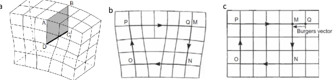
An edge dislocation is a defect where an extra half-plane (see Fig.I.12) or several extra-planes (see Fig.I.15) of atoms is introduced mid-way through the crystal. The crystalline lattice distortion is serious where the extra half plane ends. This corresponds to what is called the dislocation line (line CD in Fig.1.12(a)) or dislocation core (cylinder of small, arbitrary radius surrounding the CD line). The atoms outside the dislocation core are only elastically disturbed. An important definition of a dislocation is given in terms of its Burgers circuit. A Burgers circuit in a crystal containing a dislocation is an atom-to-atom path which forms a closed loop path as illustrated in Fig.1.12(b). If the same atom-to-atom sequence is made in a perfect crystal without dislocation, the circuit does not close Fig.1.12(c). This means that the first circuit, Fig.1.12(b), encloses a dislocation. The vector required to complete the circuit in the perfect crystal Fig.1.12(c), is called the Burgers vector of the dislocation. For an edge dislocation, the Burgers vector is normal to the line of the dislocation.

Fig. I.12 An edge dislocation (a) and the Burgers circuit (b and c). From Hull and Bacon (2011)

(27)

When a large enough shear stress is applied from one side of the crystal structure, the edge dislocation glides: the ‘extra plane’ passes through planes of atoms, breaking and producing new bonds (see Fig.I.13), until it reaches a free surface (Fig.I.13) or another extended defect. A surface step is created when the dislocation comes out of a free surface. In the first part of this work, edge dislocations will be produced by inserting extra half planes and calculating the elastic displacements of the atoms nearby. The dislocation will be driven to the free surface under a small shear stress or because of the attractive image force. This point will be explained in details later on in this chapter. We call a ‘slip system’ the ensemble of Burgers vector, dislocation line and the slip plane.

Fig. I.13. Glide of an edge dislocation and the creation of a surface step

A screw dislocation is much harder to visualize. Imagine cutting a crystal along a half-plane and slipping one-half across the other by a lattice vector, the halves fitting back together without leaving a defect except for the line defining the half plane and its surrounding core (Fig.I.14). For a screw dislocation, the Burgers vector is parallel to the line of dislocation. We refer the reader to classical textbooks for more illustrations and details. A screw dislocation in an otherwise perfect but finite crystal implies the existence of two semi-extended surface steps which will further extend if the screw dislocation moves.

Fig. I.14. A screw dislocation, with the creation of two surface steps. The AA’ line glides and reaches the BB’ position.

Shear stress

Surface step Shear stress _{Shear stress}

(28)

1.4.2 More details about dislocations in fcc metals

Our work focus on fcc metals, therefore the following focuses on dislocations in fcc structures. We use the conventional cubic crystallographic referential system, usually normalising the cubic lattice parameter to 1. In fcc crystals, the smallest Burgers vector b for perfect dislocations are ½ <110>. The atomic {110} planes are perpendicular to <110> and have a two-fold stacking sequence ABAB. The ‘extra half-plane’ for such an edge dislocation thus actually consists of two (110) atomic half planes in the ABAB sequence as shown in Fig.I.15. The dislocation core is located in a close-packed (111) type plane which is the glide plane. Dislocations glide in a (111) type close-packed plane and rarely in other planes. In reality, the two extra (110) planes do not stay immediately adjacent to each other. The dislocation separates into two dislocations which are called ‘partial dislocations’ and can be associated to shorter, partial, Burgers vectors. The original dislocation with a ½ <110> Burgers vector is called a perfect dislocation. The most important partial dislocations observed in face centred cubic metals are the so-called Shockley partials (Heidenreich and Shockley). An example of decomposition into two Shockley partials is:

1 2 [110] = 1 6 [211] + 1 6 [121̅]

Because the elastic energy of a dislocation is proportional to 𝑏2_{, this decomposition can be}

considered energetically favourable (Frank’s rule, an approximate rule): ( 𝑏_{𝑝𝑒𝑟𝑓𝑒𝑐𝑡})2 _{> ( 𝑏} 𝑝𝑎𝑟𝑡𝑖𝑎𝑙1)2+ ( 𝑏𝑝𝑎𝑟𝑡𝑖𝑎𝑙2)2 ∶ 1 2> 1 3

(29)

Shockley partials are ‘glissile’ because the partials can glide on the considered slip plane. There are also some ‘sessile’, i.e. non glissile partials in fcc metals such as Frank partials, Hirth partials and stair-rods.

In my simulations, perfect dislocations are produced by carefully introducing two extra half planes of atoms in the metal. More precisely, a pre-adapted elastic displacement field is firstly applied to all atoms of the crystal with respect to a chosen origin, Burgers vector and line orientation. Only then are two extra atomic half planes inserted in the ‘void’ created by elastic displacement field (seeFig. I.16).

Fig. I.16. Insertion of an edge dislocation.

Left: crystal subjected to the pre-adapted elastic displacement field. Right: introduction of an edge dislocation composed of two half planes.

The displacement field (𝑢𝑥 𝑢𝑦) is taken from the isotropic elastic theory, derived from the

stress field induced by one edge dislocation in an infinite body [Hirth and Lothe 1992]. Fig.I.17 shows a well-known representation of the stress field surrounding an edge dislocation. On the left half (a) of the picture, the stresses plotted on the elementary cube are shown around the dislocation. Since there is no stress component in the direction perpendicular to Fig.I.17, a two-dimensional representation is sufficient. On the right half (b), contours of stress isovalues are plotted for the normal component and the shear components of the stress tensor.

(30)

Fig.I.17 Stress field around an edge dislocation in an infinite body.

By integrating the elastic strain field, the displacement field in x direction is given below: 𝑢_𝑥 = _2𝜋𝑏 [𝑡𝑎𝑛−1 𝑦

𝑥+

𝑥𝑦

2 (1−𝑣)(𝑥2_+𝑦2₎] + C

The constant of integration is determined by the condition that 𝑢𝑥 → 0 𝑎𝑠 𝑦 → −, so

{ 𝑢_𝑥 = 𝑏 2𝜋[𝑡𝑎𝑛−1 𝑦 𝑥+ 𝑥𝑦 2 (1 − 𝑣)(𝑥2_{+ 𝑦}2₎− 𝜋 2] 𝑖𝑓 𝑥 < 0 𝑢𝑥 = 𝑏 2𝜋[𝑡𝑎𝑛−1 𝑦 𝑥+ 𝑥𝑦 2 (1 − 𝑣)(𝑥2_{+ 𝑦}2₎+ 𝜋 2] 𝑖𝑓 𝑥 > 0 Similarly, the displacement along the y direction is given below:

𝑢_𝑦 = − 𝑏 2𝜋[ 1 − 2𝑣 4(1 − 𝑣)ln(𝑥2+ 𝑦2) + 𝑥2_{− 𝑦}2 4(1 − 𝑣)(𝑥2_{+ 𝑦}2₎]

Our equations about the x direction displacement are different from the ones given in Hirth and Lothe’s book (both first and second editions).

During the molecular dynamics simulation, the atoms relax their positions through their mutual interactions. The solutions obtained in an infinite body are used to set the initial positions of the atoms. After time relaxation, the elastic displacement field in the finite box of interest is obtained. Similarly, the 𝑣 value used in the analytical solution corresponds to an isotropic elasticity value. But, the solution accounting for anisotropic cubic elasticity is obtained after relax. Further details are given in section I.5.

(31)

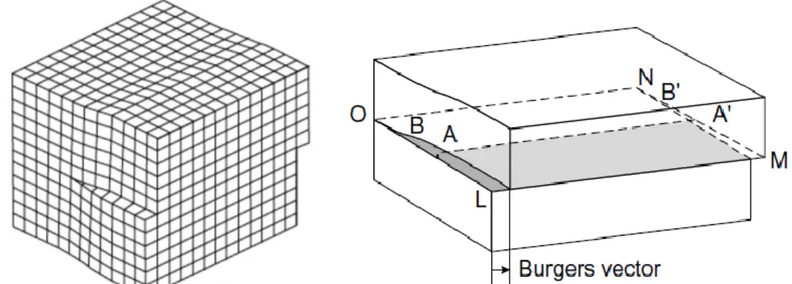
Once a perfect dislocation (made of two additional half-planes) is properly inserted, it dissociates into two Shockley partials during the molecular dynamics relaxation, confirming that the total energy of the two Shockley partials is lower than that the perfect one as previously mentioned, based on Frank’s rule. Between these two partials, a ribbon of stacking-fault is formed (Fig. I.18) which corresponds to a local staking fault between (111) atomic planes. This fault is called the intrinsic stacking fault in fcc metals. These interruptions carry a certain stacking-fault energy. The width of the stacking fault ribbon is a consequence of the balance between the ‘repulsive force’ between two partial dislocations on the one hand and the attractive force due to the surface tension of the stacking fault ribbon on the other hand. There is thus an equilibrium distance between the two partials which is related to the intrinsic stacking-fault energy value (SFE, or ISFE). As the SFE is high the dissociation is impeded, and the distance between the two partials is small. On the contrary, as the SFE is low, the distance between the two partials is large. Table 1 gives the {111} SFE of the fcc metals that we analyse in this work.

Fig. I.18 Dissociation of a b1 perfect edge dislocation into two Shockley partials of Burgers

(32)

material Ag Ni Cu Al SFE (mJ m−2) 15-211 120 44-781 143-2001 b (10-10 _m) _2.889 _2.492 _2.556 _2.915 µ (GPa) 42.9 111.3 48 25.5 µb (mJ m−2) 12.4 27.7 12.3 7.4 SFE normalized 1.21-1.69 4.33 3.58-6.34 19.32-27.03 Table I.1: Stacking fault energies of different fcc metals. In the last line of the table, the SFE is normalized by µb (normalized SFE = SFE/ µb) to facilitate the comparison between different materials (see [Seeger 1955]). b is the Burgers vector length and µ is the experimental value of isotropic shear modulus for poly-crystals without texture. 1 [Bernstein and Tadmor 2004], 2 [Murr 1975].

In fcc metals, the densest planes are the {111} planes which are thus the most favourable slip planes for dislocations. For a non-dissociated 1/2[1̅01] screw dislocation slipping in a (111) plane under a given shear stress, it may happen that at a given time or location, a local change in stress direction let that screw dislocation slip in a (11̅1) plane once that plane also contains the 1/2[1̅01]Burgers vector and line screw direction. This phenomenon is called cross-slip. If the screw dislocation is relatively rapidly set back to a (111) plane, this is naturally called a double cross-slip event. Multiple cross-slips produce wavy trajectories for the screw dislocations and wavy slip lines. As illustrated in Fig. I.19, the (111) and (11̅1) planes both contain the [1̅01] vector, so that the screw dislocation can switch from the (111) plane to the (11̅1) plane. Fig. I.19(d) shows a double cross-slip. If the screw dislocation is dissociated, its partials are no longer pure screw dislocations and cross-slip is less easy, all the less if the partials are separated by a large ribbon-fault. Nevertheless, partial dislocations are always less separated for a screw dislocation than for an edge dislocation, by a factor of about 2 [Read 1953]. Cross-slip may be locally assisted by local constrictions due to the encounter of a barrier provided by a non glissile dislocation or an impenetrable obstacle (Seeger-Escaig-Friedel mechanism). Pure fcc metals with a low SFE (or SFE / (𝜇b)) are thus less prone to cross-slip than metals with a high SFE. The latter are called ‘wavy’ materials, the former are called ‘planar’ materials [McEvily and Johnston 1967]. Aluminium, copper and nickel, are wavy materials. Let us note that for alloys the low SFE/(𝜇b) criterion does not work in cases of short range order, see [Clément 1984].

In wavy materials, annihilation of dislocations is favoured by cross slip. This will of course induce a high irreversibility of dislocation motions. The concept of irreversibility is defined and used in details in chapter II.

(33)

Fig. I.19. Illustration of a cross-slip (a,b,c) and a double cross-slip (d). From [Hull and Bacon 2011].

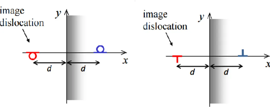
1.4.3 Image forces

Once a dislocation is close to a free surface, it can be attracted to the surface by the so called image force whose origin is explained below.

The elastic energy of a dislocation is the elastic energy associated to the elastic displacement field caused by the dislocation around itself. Beyond the free surface, where there are no atoms, there is no elastic displacement field, hence no elastic energy. Thus, the closer a dislocation is to a free surface, the smaller the elastic energy it causes in that direction. This corresponds to an attractive force towards the free surface. One can show that this force is equivalent to the force which would be exerted on the dislocation by an image dislocation with respect to the surface plane, hence the expression ‘image force.’ This image trick allows for analytical calculations in very simple cases, e.g. for an edge dislocation whose line is parallel to the surface plane. Unfortunately, however, it is not helpful for more complex geometries (beyond those considered by Jens Lothe in [Indenbom 1992]). It remains that a dislocation is attracted by a free surface. In my simulations, I sometimes intentionally put dislocations near a free surface, so that the emergence of dislocations on the surface can be observed spontaneously without applying any stress to the system.

(34)

Fig. I.20. Image dislocation of a screw (left) and an edge (right) dislocation near a free crystalline surface.

1.5 Computer simulations

Computer simulation is widely used to model atom behaviour in crystals and provide information not easily accessible by experimental investigation. In this study, Molecular Dynamics (MD) simulations are carried out which allow us to follow the trajectories of atoms in real time. Basic literature on the subject includes: Allen and Tildesley 1987 and 1989, Frenkel and Smit 1996, Ciccoti, Frenkel and McDonald, 1987, Meyer and Pontikis 1991, Kirchner, Kubin and Pontikis 1995. Both homemade programs (from my PhD supervisor O. Hardouin Duparc) and the Large-scale Atomic/Molecular Massively Parallel Simulator (LAMMPS) [http://Lammps.sandia.gov] software are used. MD simulations with LAMMPS allow simulating atomic system up to a hundred nano-meters in size during times up to several nanoseconds (Fig. I.21).

(35)

The potential energy of the model system and the forces between the atoms are computed from interatomic potentials. As forces are usually deduced from interatomic potentials, ‘Force Field’ is mainly another name for ‘interatomic potential’ (except for ab initio modelling). Such potentials for austenitic steels and nickel based alloys are still in development in 2016. Thus only pure fcc metals are investigated in this work for which reliable interatomic potentials exist. The work of [Bernard et al. 1987] shows that the mechanisms of fatigue damage under a large number of cycles in austenitic steels are rather similar with the copper ones because of the common crystallographic structure. Therefore, investigations with pure fcc metals can be useful and necessary to ensure a better understanding of mechanisms at atomic level. Furthermore, many measurement and observation results are available for copper and nickel whose fatigue mechanisms have been widely studied. These will help us to compare our simulation results with experimental data. Finally, the behaviours of both a low stacking fault energy metal, silver, and a high SFE metal, aluminium, are investigated too. The SFE of austenitic stainless steels is about 20-30 mJ/m2, between the silver and copper values.

Reliable interatomic potentials are available for the four fcc materials investigated in this work: aluminium, copper, nickel and silver. The interatomic potentials mostly used for simulations in inert environment are so called Embedded Atom Model (EAM) potentials. Their empirical parameters are adjusted for prediction of material parameters such as cohesive energy, elastic constants, phonon spectra, point defect energies, surface energies and stacking fault energies, as close as possible to measured values or values derived from ab initio calculations. Some smaller scale ab-initio (DFT) simulations have thus been carried out to compare with values estimated by EAM potentials. I used the Vienna Ab initio Software Program (VASP) for these calculations, based on the density functional theory (DFT). Reference books give the required background [Martin 2008; Thijssen 1999; Thijssen 2013]. All the potentials I used give rather good estimations of the physical parameters of the investigated fcc metals. For the simulations carried out in oxygen environment, in order to simulate the chemical reactions of the oxygen molecules with the metals, such as their dissociation into oxygen atoms, I used Reactive Force Fields (ReaxFF) such as those developed by van Duin and co-workers. I also used the COMB (Charge-Optimized-Many-Body) potential which is another force field that allows the simulation of interactions between metal and oxygen.

(36)

It should be noticed that the potentials I used also reproduce accurately the unstable stacking fault energy of the metals. The unstable stacking fault energy is an influent parameter linked to the energy barrier for partial dislocation nucleation. The potentials are therefore able to reflect both dislocation nucleation and interaction phenomena. That is required for answering the irreversibility of surface slips and the crack tip behaviour. More details about EAM potentials are given in chapter 2 and some details about ReaxFF and COMB potentials are given in chapter 3.

In molecular dynamics, at a given instant of time t, the acceleration of every atom is calculated from the total force on it due to its neighbours using Newton’s second law (force = mass times acceleration, f(t)=mγ(t)). The computer codes use this equation to predict the evolutions of the positions of all atoms with time. With a finite time difference algorithm such as the Verlet algorithm: 𝑥(𝑡 + 𝛿𝑡) = 2𝑥(𝑡) − 𝑥(𝑡 − 𝛿𝑡) +𝑓(𝑡)_𝑚 𝛿𝑡2_{+ 𝑜(𝛿𝑡}4_{), where 𝛿t is the}

molecular dynamics finite difference time-step. To maintain numerical stability and convergence, the time step 𝛿t is typically of the order of one femtosecond.

In some applications, one just wants to find the ground state atom coordinates of a system, for example, minimize the total energy to the nearest energy minimum, this is called molecular statics. In molecular statics, the kinetic energy of the atoms is scaled down to zero, and the system achieves equilibrium as the potential energy is minimized. In our simulations, we do this once an edge dislocation is inserted and the displacement field is pre-calculated and applied (see I.4.2). This process helps to relax the dislocation configuration and to make sure that all atoms are in lower energy positions before running molecular dynamics.

The typical time-step of MD simulation is from one to several femtoseconds, the number of time-steps that can be accomplished within a reasonable computer time during a PhD work for systems containing several hundreds of thousands of atoms is typically in the range 105 to 107. As a consequence, the total simulated time is limited to the order of nanoseconds. This has consequences on the strain rates that we apply: their orders of magnitudes are much higher than the strain rates experimentally applied. Yet, extrapolations which are possible for some simulations show that the results are still valid until the order of second. In our largest simulation box, almost 2,000,000 atoms are simulated. Periodic boundary conditions are applied for most simulations. Sometimes, however, in order to allow the oblique glide along

(37)

some of the slip systems, periodic boundary conditions are relieved. In this case, some thin foil artefacts could be introduced but these artefacts can correspond to nano thin foils. Otherwise, one has artefacts due to the use of periodic boundary conditions, which do not exist in most of materials. Further assessments will be developed in chapter 4.

The OVITO [https://ovito.org/] software is applied in the post-processing of LAMMPS outputs. OVITO is a visualization and analysis tool which can detect point defects, dislocations, different crystallographic structures, stacking faults, etc.

(38)

CHAPTER 2. SURFACE STEP IRREVERSIBILITY & CRACK

INITIATION IN INERT ENVIRONMENT

In the first part of this PhD work, surface slip irreversibility is analysed in inert environment. In ductile metals, fatigue damage generally starts at free surfaces. Experiments demonstrate that removing the surface roughness by electro-polishing leads to an increase in total fatigue life [Suresh 1998]. Since the classical work on the fracture of metals under alternated stress by [Ewing and Humfrey 1903], when dislocations were not known for crystals, it is now accepted that the initiation of fatigue cracks at free surfaces often arises from the accumulation of unreversed slip steps. Cyclic micro-plasticity based on the glide of dislocations is one of the mechanisms responsible for the fatigue phenomena in single phase fcc metals and alloys. Irreversibility mechanisms appear to be crucial to understand fatigue microcrack initiation and propagation. Glide irreversibility can be characterized by the fraction p of irreversible plastic slip per cycle compared to the total plastic slip (p=γplirr/γpl)

[Woods 1973; Mughrabi et al. 1979]. This slip irreversibility p amounts to zero if slip is entirely reversible, and it reaches one if slip is entirely irreversible. Hence, 0≤ p ≤ 1. Qualitatively, short and long fatigue lives can be expected to be related to large and small values of the glide irreversibility p respectively. Experimental studies of p are usually carried out by direct measurements on surfaces. Analytical models in the literature usually estimate p based on dislocation motions in the bulk and neglect surface mechanisms. A precise description of the surface irreversibility is certainly necessary. The aim of this work is to evaluate random surface step irreversibility by atomistic analyses of surface step evolution mechanisms in order to ameliorate the bulk irreversibility models by explicitly taking into account the mechanisms of surface steps.

(39)

2.1 Literature review on experimental observations and irreversibility models

It is generally accepted that fatigue crack initiation occurs at sites of stress concentration caused by the surface relief evolution of emerging persistent slip bands (PSBs). [Cheng and Laird 1981] further found that, in copper, fatal cracks preferentially form at the PSBs with the largest local strain. The occurrence of fatigue-induced slip bands was noted for the first time in 1903 by Ewing and Humfrey. Fifty years later, [Thompson et al. 1956] showed that the slip bands are persistent in the sense that they always re-appear at the same places after repolishing-recycling sequences. These slip bands are thus called ‘persistent slip bands’ (PSBs). Since then, many efforts in the field have been dedicated to the study of the PSBs in the bulk. Studies were first mainly performed on copper crystals [Watt et al. 1968; Basinski et al. 1969; Winter 1973; Finney and Laird 1975; Finney and Laird 1982; Basinski et al. 1983], and also, more recently, nickel single and polycrystals [Mecke and Blochwitz 1982; Hollmann et al. 2000; Weidner et al. 2006; Weidner et al. 2008; Holste 2004]. When the cyclic loading amplitude is under the PSB slip threshold, the microscopic structure contains relatively few dislocations and is rather homogeneous (Fig. II.1a). When the deformation approaches the PSB threshold, instability of the microstructure induces the formation of PSBs (Fig. II.1b) which have the so-called ‘ladder structure’ [Winter 1973; Mughrabi et al. 1979]. There are plenty of edge dislocations in the dark “walls” whereas the screw dislocations glide in the ‘channels’ between the walls. Edge dislocations glide from one wall to the next one.

Fig. II.1 Microstructure evolution under cyclic loading in copper. a) load under the PSB slip threshold, b) load higher than PSB threshold, ladder structure of PSB. Image (a) is from [Woods 1973] and image (b) is from [Mughrabi et al. 1979] (also see fig.1 of [Winter 1973]).

(40)

The threshold amplitude for the formation of PSBs has been related in the past to the existence of a true fatigue limit [Mughrabi and Wang 1981; Mughrabi et al. 1991; Laird 1976]. In polycrystals, it has also been clarified that these thresholds represent only the condition for initiation of stage I shear micro-cracks but do not necessary fulfill the conditions for subsequent propagation of these cracks [Mughrabi et al. 1991; Mughrabi and Stanzl-Tschegg 2007; Stanzl-Tschegg and Schönbauer 2007]. Hence, according to these studies, the true fatigue limit actually lies somewhere above the thresholds for PSB formation.

Fig. II.2. Example of optical micrograph of taper section of fatigued copper polycrystal, showing ‘‘notches and peaks’’ forming at the head of a slip band [Wood 1958].

In the early studies, [Wood 1958] showed with the ‘taper sectioning’ technique that the specimen surface roughens rapidly within the PSB’s, thus indicating that a considerable fraction of the cyclic slip in the PSB’s must be irreversible. Wood observed that cracks initiate in the notch-peak surface geometry formed by to-and-fro displacement. [May 1960] formulated the idea of the crack initiation as a consequence of random irreversible slip events. The experimental studies carried out by [Hull 1957] and by [Cottrell and Hull 1957] on copper single and poly crystals showed that the surface relief also developed at very low temperature down to 4.2K, indicating that the evolution of the surface relief could be a pure mechanical mechanism. Numerous models [Cottrell and Hull 1957; Mott 1958; Kennedy 1963; Watt et al. 1968; Woods 1973; Mughrabi et al. 1979; Essmann et al. 1981; Essmann 1982; Differt et al. 1986; Mughrabi 2009; Mughrabi 2010] have been proposed to interpret experimental observations.

A well-known model which describes the evolution of the surface roughness for fcc metals has been developed by Essmann, Gösele, Mughrabi and Differt (EGM or EGDM model)