Textmining without document context.

HAL Id: hal-00636111

https://hal.archives-ouvertes.fr/hal-00636111

HAL is a multi-disciplinary open access

archive for the deposit and dissemination of sci-entific research documents, whether they are

pub-L’archive ouverte pluridisciplinaire HAL, est destinée au dépôt et à la diffusion de documents scientifiques de niveau recherche, publiés ou non,

Textmining without document context.

Eric Sanjuan, Fidelia Ibekwe-Sanjuan

To cite this version:

Eric Sanjuan, Fidelia Ibekwe-Sanjuan. Textmining without document context.. Information Pro-cessing and Management, Elsevier, 2006, 42 (6), pp.1532-1552. �10.1016/j.ipm.2006.03.017�. �hal-00636111�

Text mining without document context

Eric SanJuan

_{Fidelia Ibekwe-SanJuan}

a_{LITA, Universit´e de Metz & URI, INIST-CNRS}

Ile du Saulcy, 57045 Metz Cedex 1, France

b_{URSIDOC-ENSSIB & Universit´e de Lyon 3}

4, cours Albert Thomas 69008 Lyon Cedex, France

Abstract

We consider a challenging clustering task: the clustering of muti-word terms without document co-occurrence information in order to form coherent groups of topics. For this task, we developed a methodology taking as input multi-word terms and lexico-syntactic relations between them. Our clustering algorithm, named CPCL is implemented in the TermWatch system. We compared CPCL to other existing clustering algorithms, namely hierarchical and partitioning (k-means, k-medoids). This out-of-context clustering task led us to adapt multi-word term representation for statistical methods and also to refine an existing cluster evaluation metric, the editing distance in order to evaluate the methods. Evaluation was carried out on a list of multi-word terms from the genomic field which comes with a hand built taxonomy. Results showed that while k-means and k-medoids obtained good scores on the editing distance, they were very sensitive to term length. CPCL on the other hand obtained a better cluster homogeneity score and was less sensitive to term length. Also, CPCL showed good adaptability for handling very large and sparse matrices.

Key words: Multi-word term clustering, lexico-syntactic relations, text mining, informetrics, cluster evaluation.

1 Introduction

We developed a fast and efficient text mining system that builds clusters of noun phrases (multi-word terms) without need of document co-occurrence

in-Email addresses: [email protected], [email protected] (Fidelia Ibekwe-SanJuan).

formation. This is useful for mapping out research topics at the micro-level. Because we do not consider the within document co-occurrence, our approach can be conceived as an out-of-context clustering except if we consider the intra-term context, i.e., words appearing in the same intra-terms can be said to share a similar context. Terms are clustered depending on the presence and number of shared linguistic relations. For instance, a link will be established between the two terms humoral immune response and humoral Bhx immune response since one is lexically included in the other. Likewise clustering algorithm is linked to computer algorithm by a modifier substitution. This lexico-syntactic approach is suitable for clustering multi-word text units which rarely re-occur as is in the texts. Such multi-word terms (MWTs) often result in very large and sparse matrices or graphs1 _{that are difficult to handle by the existing} approaches to clustering which rely on high frequency information. The re-sulting system, called TermWatch (Ibekwe-SanJuan, 1998a; Sanjuan et al., 2005) can be applied to several tasks like domain topic mapping, text mining, query refinement or question-answering (Q-A).

Some attempts have been made to cluster document contents in the biblio-metrics, scientometrics and informetrics fields. Some authors have considered the clustering of keywords, classification codes or subject headings assigned to documents by indexers (Callon et al., 1991; Zitt and Bassecoulard, 1994; Braam et al., 1991). Although these information units depict the thematic contents of documents, they are external to the documents themselves and do not allow for a fine-grained analysis of the current topics addressed in the full texts. In studies where the document contents were considered, only lone words were extracted through statistical analysis. The majority of clustering methods used in the information retrieval field (Eisen et al., 1998; Cutting et al., 1992; Karypis et al., 1994) are also based on the vector-space represen-tation model of documents (bag-of-words approach). To reduce the dimensions of the vector space, words with a discriminating power are selected based on term weighting indices like the Inverse Document Frequency (IDF), Mutual Information (MI) or the cosinus measure. This also results in the drastic elim-ination of more than half of the initial data from the analysis. Our text mining approach treats highly frequent and low frequent terms equally. This is impor-tant for applications like science and technology watch where the focus is on novel information often characterised by low frequency units (weak signals). Price and Thelwall (2005) have demonstrated the usefulness of low frequency words for scientific web intelligence (SWI). They showed that removing low frequency words reduced cluster coherence and separation, i.e., clusters were less dissimilar.

Glenisson et al. (2005) proposed combining full text analysis with bibliometric 1 _{In the experiments run up to date, we have been able to handle graphs of 80, 000}

analysis in order to cluster the research themes of 85 scientific papers. Text contents were represented as vectors of lone words. Stemming was performed on the words and bigrams were detected, i.e. sequences of two adjacent words that occurred frequently. It is a well known fact that stemming brutally re-moves the semantics of derived or inflected words. For instance, “stationary, station, stationed ” are all reduced to station. Also, bigrams may not always correspond to valid domain terms. The authors weighted the bigrams using the Dunning likelihood ratio test (Dunning, 1993). This led to selecting the 500 topmost bigrams for analysis and discarding the rest. One of the interest-ing findinterest-ings of this study is that clusterinterest-ing items from full texts rather than keywords or terms from the reference section leads to a more fine-grained and accurate mapping of research topics. This finding is in line with our text mining approach.

Polanco et al. (1995) developed the Stanalyst informetrics platform. Stan-alyst comprises a linguistic component which identifies variants of MWTs used to augment their occurrences. The MWTs are then clustered based on document co-occurrence information. To the best of our knowledge, no infor-metric method has considered clustering phrases based on linguistic relations. The TermWatch approach is based on the hypothesis that clustering multi-word terms (MWTs) through lexico-syntactic and semantic relations can yield meaningful clusters for various applications. In view of this, we developed a methodology that can handle very large and sparse matrices in real time. For instance, in the current experiment, the input list of terms is 31, 398, none which is eliminated prior to the matrix reduction phase.

The clustering algorithm implemented in TermWatch is named CPCL (Clas-sification by Preferential Clustered Link). This algorithm was first published in (Ibekwe-SanJuan, 1998a) but owing to its fundamental differences with ex-isting approaches, setting up an adequate comparison framework with other methods has been a bottleneck issue. In this paper, we focus on the evalua-tion with other clustering algorithms (variants of partievalua-tioning and hierarchical algorithms). Evaluation is carried out on a test corpus (the GENIA project) which comes with an answer key (gold standard). This will ensure that the results being presented are grounded in the real world.

The rest of the paper is organised as follows: section 2 gives details of the test corpus; section 3 describes our text mining methodology; section 4 presents the evaluation method; section 5 describes the experimental setup; section 6 discusses the results of the evaluation with other clustering methods; section 7 draws remarks and conclusions.

2 Test corpus

In order to carry out an evaluation, we chose a dataset with an existing ideal partition (gold standard). The GENIA project2

consists of 2, 000 abstracts downloaded from the MEDLINE database using the search keywords: Hu-man, Blood Cells, and Transcription Factors. Biologists manually annotated the valid domain terms in these texts, yielding 31, 398 terms. This ensures in our experiment that competing methods start from the same input. The GENIA project also furnished a hand-built ontology, i.e. a hierarchy of these domain terms arranged into semantic categories. There are 36 such categories at the leaf nodes. Each term in the GENIA corpus was assigned a semantic category at the leaf node of the ontology. We shall refer to the leaf node cat-egories as classes henceforth. Of course, the GENIA ontology’s hierarchy, the number of classes and the semantic category of each term were hidden from the clustering methods. It should be noted that since the GENIA ontology is a result of a human semantic and pragmatic analysis, we do not expect automatic clustering methods to reproduce it exactly without prior and ad-equate semantic knowledge. The goal of the evaluation is to determine the method whose output requires the least effort to reproduce the classes at the leaf nodes of the ontology. Also, it is worth noting that although the authors of this project use the term ontology to qualify this hierarchy, it is more of a small taxonomy. Indeed, the GENIA ontology is still embryonic because of its small size (36 classes, 31, 398 terms). The classes are of varying sizes. The largest class, called other name has 10, 505 terms followed by the protein molecule class with 3, 899 terms and the dna domain or region class with 3, 677 terms. The 12 smallest classes ( rna domain or region inorganic, rna substructure, nucleotide, atom, dna substructure, mono cell, rna n/a, protein n/a, carbo-hydrate, dna n/a, protein substructure ) each has less than 100 terms. It is quite revealing that the largest class is a miscellaneous class. This suggests that this class can be further refined. Also some relations normally found in a full-fledged ontology are absent (synonymy in particular). This tends to sug-gest that this hierarchy is a weaker semantic structure than an ontology and can thus constitute an adequate clustering task. For these reasons, we prefer to refer to it as the GENIA taxonomy henceforth.

Table 1 gives some examples of terms in the GENIA corpus.

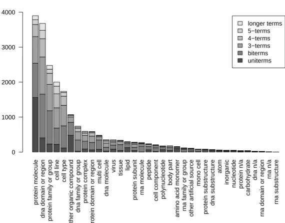
Figure 1 shows the fast decreasing distribution of terms in the 35 classes. We omitted the largest class, called other name which concentrated 33% of the terms because it was difficult to fit in. A few number of classes (protein molecule, dna domain or region, protein family or group, cell line, cell type) concentrated the rest of the terms (almost 75%). The bars show the proportion 2 _{http://www-tsujii.is.s.u-tokyo.ac.jp/GENIA/.}

GENIA Category Terms

amino acid monomer amide-containing amino acidasparagine n-acetylcysteine

atom cytosolic calcium

feca2+ body part

organ

peripheral lymphoid organ tumor-draining lymph node

cell component

1389 sites/cell

b6d2f1 mouse uterine cytosol cytoplasmic protein extract

il-13-treated human peripheral monocyte nuclear extract cell line

anergized t cell

adherence-isolated monocyte xenopus hepatocyte

other name

anatomic tumor size apoptosis

follicular lymphoma Table 1. Examples of terms in GENIA corpus

of terms according to their length. As a consequence of this fast decreasing model, a clustering method optimised for one of the prominent classes can obtain good scores without correctly classifying terms in the majority of the smaller classes. Another feature that can be observed in figure 1 is that the distribution of one word terms is not correlated with the general distribution of terms. Meanwhile, we will see in section §6 that most of the clustering methods perform better on long terms and thus on classes like “protein family or group” and “dna domain or region” that contain few one word terms. In an OTC task, the intrinsic properties of MWTs (like term length) obviously play an important role since they are the only available context.

3 Overview of our text mining methodology

Our methodology consists of three major components: MWT extraction; re-lation identifier and clustering module. An integrated visualisation package3 can be used if topic mapping is the target. In this experiment, this aspect will not be explored as evaluation will focus on cluster quality and not on their 3 _{The aiSee visualization package (http://www.aisee.com) has been integrated to}

protein molecule dna domain or region _{protein family or group}

cell line _{cell type}

other organic compound

dna family or group

protein complex

protein domain or region

multi cell

dna molecule

virus

tissue lipid

protein subunit rna molecule

peptide

cell component polynucleotide

body part

amino acid monomer

rna family or group

other artificial source

mono cell

protein substructure

dna substructure

atom

inorganic

nucleotide protein n/a

carbohydrate

dna n/a

rna domain or region

rna n/a rna substructure longer terms 5−terms 4−terms 3−terms biterms uniterms 0 1000 2000 3000 4000

Fig. 1. Distribution of terms in GENIA categories.

layout. However, interested readers can find an application of research topic mapping in (Ibekwe-SanJuan and SanJuan, 2004).

3.1 Term extraction module

Note that in the current experiment, our term extraction module was not used as the terms were already manually annotated in the corpus. We however de-scribe summarily its principle. TermWatch performs term extraction based on shallow natural language processing (NLP) techniques. Extraction is imple-mented via the NLP package developed by the University of Edinburgh. LT-POS is a probabilistic part-of-speech tagger based on Hidden Markov Models. It uses the Penn Treebank tag set which ensures the portability of the tagged texts with many other systems. LTCHUNK identifies simplex noun phrases (NPs), i.e., NPs without prepositional attachments. In order to extract more complex terms, we wrote contextual rules to identify complex terminological NPs. An example is provided in appendix A. About ten such contextual rules were sufficient to take care of the different syntactic structures in which nom-inal terms appear in English. Given that some domain concepts can appear

as long sequences like in parental granulogyte-macrophage colony-stimulating factor (GM-CSF)-dependent cell line, it is obvious that such MWTs are not likely to re-occur frequently in the corpus. Hence, the difficulty of clustering them with methods based on co-occurrence criteria.

3.2 Relation identifier

Different linguistic operations can occur within NPs. These operations either modify the structure or the length of an existing term. They have come to be known as variations and have been well studied in the computational termi-nology field (Jacquemin, 2001; Ibekwe-SanJuan, 1998b). Variations occur at different linguistic levels: morphological (gender and spelling variants), lexical (substitution of one word by another in an existing term), syntactic (expansion or structural transformation of a term), semantic (synonyms, generic/specific relations). Our relation identifier tries to acquire all these types of variations among the input terms.

3.2.1 Morphological variants

These refer to number (tumor cell nuclei /tumor cell nucleus) and gender variations in a term and also to spelling variants. They enable us to recog-nise different appearances of the same term. For instance, IL-9-induced cell proliferation will be recognised as a spelling variant of IL 9-induced cell pro-liferation. Spelling variants are identified using cues such as special characters while gender and number variants are identified using WordNet ((Fellbaum, 1998)

3.2.2 Lexical variants

We call substitution variants operations involving the change of only one word in a term, either in the modifier position (coronary heart disease ↔ coronary lung disease) or in the head position (mutant motif ↔ mutant strain). The head is the noun focus in an English NP, i.e., the subject while the modifier plays the role of a qualifier (an adjective). The head word is usually the last noun in a compound phrase (strain in mutant strain) or the last noun before a preposition in a prepositional structure (retrieval in retrieval of information).

3.2.3 Syntactic variants

These refer to the addition of one or more words to an existing term as in information retrieval and efficient retrieval of information. We call these

op-erations expansions. Expansions that affect the modifier words are further broken down into left-expansion and insertion. Alternatively, expansions can affect the head word. In this case, we talk of right expansion.

Morphological variants (spelling) and permutation variants are recognised first since they refer to the same term. Then these variants are used to recognise the more complex variants. For instance, B cell development haven been recog-nised as a spelling variant of B-cell development, this enables the identification of other types of variants (syntactic and lexical) containing the two spelling variants. Variations are assigned a role during clustering depending on their interpretation. This will be further detailed in section §5.

3.2.4 Semantic variants

It is an accepted fact that syntactic relations suggest semantic ones (left ex-pansions and insertion can engender generic-specific links, some substitution variants can reflect see also relations). However, these semantic relations are not explicit. Moreover, the types of relations considered so far all require one stringent condition: that the related terms share some common words. This leaves out terms which can be semantically-linked but without sharing com-mon words, i.e. synonyms. In order to acquire explicit semantic links, we need an external semantic resource. For this purpose, we chose WordNet (Fellbaum, 1998), a large coverage semantic database which organises English words into synsets. A synset is a particular sense of a given word. Since WordNet organises only words and not multi-word terms, we had to devise rules in order to map word-word semantic relations into “MWT- MWT” relations in our corpus. One way to achieve this is to replace words by their synsets and then apply the same variation relations to sequence of synsets. However, like all external resources, WordNet has some limitations. First is its incompleteness vis-`a-vis specialised domain terminology. Second, being a general purpose semantic database, WordNet establishes links which can be incorrect in a specialised domain.

We thus restricted the use of WordNet to filtering out lexical substitutions, and consequently to pairs of terms that share at least one word in order to reduce the number of wrong semantic links. Only a very few number of relations were found. The following rule was applied to lexical substitutions in order to identify the semantic ones using WordNet hierarchy: given two terms related by a lexical substitution, check if the two words substitued are linked by an ascending or descending path in the hierarchy. Observe that, by definition of lexical substitutions, this rule ony applies to words that are in the same grammatical position (head or modifier).

T cell growth ∼ T cell maturation

antenatal steroid treatment ∼ prenatal steroid treatment

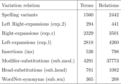
Only 365 WordNet modifier substitutions and 208 WordNet head substitutions were found whereas lexico-syntactic variants were much more abundant (see table 2 below).

Table 2 gives the number of variants identified for each type among the GENIA terms. As a term can be related to many others, the number of relations is always higher than the number of terms.

Variation relation Terms Relations

Spelling variants 1560 2442

Left Right-expansions (exp 2) 294 441 Right-expansions (exp r) 2329 3501

Left-expansions (exp l) 2818 4260

Insertions (ins) 526 798

Modifier-substitutions (sub mod.) 4291 37773 Head-substitutions (sub head) 781 1082

WordNet-synonyms (sub wn) 365 208

Table 2. Statistics on variation relations per type

Details of the variation identification rules are given in Appendix B.

3.3 Clustering module

The TermWatch system implements a graph-based approach of the hierar-chical clustering called CPCL (Classification by Preferential Clustered Link) originally introduced by Ibekwe-SanJuan (1998b). The main features of this approach are :

(1) the intuitiveness of its results for human users since any pair of terms clustered together are related by a relative short path of real linguistic relations,

(2) an ultrametric model that ensures the existence of a unique and robust solution,

(3) its linear time complexity on the number of variations that allows inter-active data analysis since clustering can be processed in real time.

We show here that this algorithm can be applied to other types of inputs. For that, we need to cast the description of the algorithm in the more general context of data analysis.

Let S be a sparse similarity data matrix defined on a set Ω of objects. This matrix can be represented advantageously by a valuated graph G = (Ω, E, s) where E is the set of edges made of all unordered pairs {i, j} of objects such that Sij > 0 and s is the valuation of edges defined for all (i, j) ∈ Ω2

by s(i, j) = Sij. In the case of sparse data, the size of E is much smaller than |Ω|2

.

Let V alS be the set of values in S. If |V alS| ¿ |S| then, the usual hierarchical algorithms will produce small dendrograms since they will have at most |V alS| levels. Thus, they will induce a very reduced number of intermediary balanced partitions in the gap between the trivial discrete partition and the family of connected components of G. A way to correct this drawback of hierarchical clustering without losing its intuitiveness and computer tractability is not to consider edge values in an absolute way but in the context of adjacent edges. Thus, two objects related by an edge e will be clustered at a given iteration, only if the value of e is greater than any other value in its neighborhood. This means that i, j will be clustered at the first iteration only if Sij is greater than the maximum in the line Si. and in the column S.j. It has been shown in Berry et al. (2004) that this variant of hierarchical clustering preserves its main ultrametric properties.

This solution is specially well adapted when the observed similarities between objects are generated by pairwise observations. In the case of out-of-context clustering (OTC), given three terms u, v, t such that v shares at least one word with u and t (possibly not the same), we will consider a local criteria to decide if v is closest to u or to t.

In this approach, the clustering phase can be easily implemented using the following straightforward procedure which we call SLM E ( Select Local Max-imum Edge). This procedure runs in linear time on the number of edges. In fact, the procedure does as many comparisons as the sum of vertex degrees which is two times the number of vertices. It uses a hash table m to store, for each vertex x, the maximal value of previously visited adjacent edges.

SLME procedure

Input : a valued graph (V,E,s) Output : a relation R on V L:={}

for every x in V, m[x] := -1 while V-L is not empty

Select one vertex v in V-L add v to L

C:={v}

while C is non empty x:=pop(C)

add x to L

add neighbours(x) - L to C

m[x] := max{s(n): n in neighbours(x)} for every n in neighbours(x)

if m[n]=m[x] add {n,x} to R

Once done, the clustering phase consists in computing the reduced graph G/R, whose vertices are the connected components of the subgraph (V, R) of G and in inducing a new valuation according to a hierarchical criteria chosen among the following:

single-link: the value of an edge in G/R between two components C1, C2 is the maximal value of edges in EC1,C2 = E ∩ (C1× C2).

complete-edge: the minimal value in EC₁C2,

average-edge: the average value in EC₁C₂,

vertex-weight: the sum of values in EC1C2 over |C1| + |C2|

Observe that the above complete-edge and average-edge criteria differ from the usual complete and average link clustering since they are computed on a restricted set of pairs. The vertex-weight criterion is the one that best min-imised the chain effect in our experiments. However in general, single link will also be satisfactory because the chain effect has already been reduced by the SLME procedure. In fact, this approach appears to be robust with regard to the clustering criteria. It is more sensitive to the existence of very small values in the similarity matrix S. Indeed, any non null value will generate an edge in the graph and if this edge is the only one linking two objects, then these objects will be clustered even if the similarity is very small. This drawback can be corrected by the use of a threshold which clarifies the borderline between null values and significant similarities.

The CPCL algorithm then becomes: Algorithm CPCL

input : a valued graph G=(V,E,s)

parameters : a threshold t and a number of iterations I output : a partition of V

for i=1 to i=I do

E’:= {e in E : v(e) > t} R := SLME(V,E’,s)

G := G/R return V

It involves I calls to the SLME procedure on the current reduced valued graph (V,E’,s).

It follows from this re-exploration of CPCL that it can by used for fast clus-tering of sparse similarity matrix with a reduced range of distinct values. Until now, this algorithm has been applied to the following similarity matrix defined on groups of objects and generated in two steps:

Step1: we consider a reduced subset of variation relations among those pre-sented in subsection 3.2 that we shall note COM P .

We then compute the set of connected components generated by the COM P relations. Terms that are not related by any of the variations in COM P will form singleton components.

Step2: We select a second subset of variations denoted by CLAS to group components. Next, given two components C1 and C2, a similarity value v is defined in the following way:

v = X

R∈CLAS

|R ∩ C1× C2| |R|

This similarity relies on the number of variations across the components and on the frequency of the variation type which on a large corpus will substantially reduce the influence of the most noisy variations like lexical substitutions on binary terms. The resulting matrix has all the characteris-tics that justify the application of the CPCL algorithm.

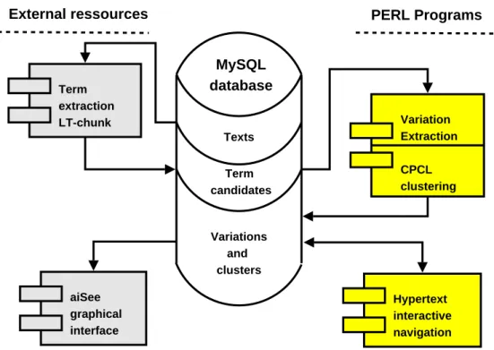
3.4 Implementation issues

Figure 2 gives an overall view of the system. It is currently run on-line on a Linux Apache MySQL Php PERL Secured (LAMPS) server4_{. The three} components term extractor, relation identifier and clustering module are im-plemented as PERL5 OO programs while all the data are stored in a MySQL database. Clustering outputs can be accessed either via an integrated visuali-sation package (aiSee based on Graph Description Language) for domain topic 4 _{TermWatch is available for research purposes after obtaining an account and a}

mapping or through an interactive hypertext interface based on PERL DBI and CGI packages. This interactive interface enables the user to browse the results, from the term network(variation links) to clusters contents and finally to documents where the terms appeared. The systems’ modules can also be executed from this interface.

Term extraction LT-chunk Hypertext interactive navigation Variation Extraction CPCL clustering aiSee graphical interface PERL Programs External ressources MySQL database Texts Term candidates Variations and clusters

Fig. 2. Overall view of the TermWatch system

4 Evaluation metrics

Evaluating the results of a clustering algorithm remains a bottleneck issue (Yeung and Ruzzo, 2001; Jain and Moreau, 1987; Tibshirani et al., 2000). The objective of the evaluation for our specific task : clustering multi-word terms out-of-context, is detailed in §4.1 followed by a review of existing evaluation methods §4.2. Finally, in §4.3 we propose enhancements to the editing distance suggested by Pantel and Lin (2002) for cluster evaluation.

4.1 Out-of-context Term Clustering (OTC)

Given a list of terms, the task consists in clustering them using exclusively surface lexical information in order to obtain coherent clusters. In this frame-work, clustering is done without contextual document information, without

any training set and in a completely unsupervised way. We refer to this task as OTC (Out-of-context Term Clustering).

Let us emphasise that OTC is different from Entity Name Recognition (ENR). ENR task as described in Kim et al. (2004) is based on massive learning tech-niques and new terms are forced to enter known categories. Whereas in un-supervised clustering, a new cluster can be formed of terms not belonging to an already existing category. This can lead to the discovery of new domain topics. It should also be noted that MWTs cannot be reduced to single words. Unlike single words, a MWT can occur only once “as is” (without variations) in the whole corpus. It is thus difficult for the usual document × feature rep-resentation to find enough frequency information to form clusters. Therefore methods based on term-document representation cannot be directly applied to OTC without adaptation. This adaptation is described in further details in §5.

4.2 Existing measures for cluster evaluation

Cluster evaluation generally falls under one of these two frameworks:

(1) intrinsice evaluation: evaluation of the quality of the partitions vis-`a-vis some criteria.

(2) extrinsic evaluation : task-embedded evaluation or evaluation against a gold standard.

Intrinsic evaluation, also called “internal criteria” is used to measure the in-trinsic quality of the clusters in the absence of an external ideal partition. Internal criteria concern measures like cluster homogeneity and separation, or the stability of the partitions with respect to sub-sampling (Hur et al., 2002). Alternatively, the measure can also seek to determine the optimal number of clusters (Hur et al., 2002).

Extrinsic evaluation, also known as “external criteria” refers to the comparison of a partition against an external ideal solution (gold standard) (Milligan and Cooper, 1985; Jain and Moreau, 1987) or a task-embedded evaluation. The comparison with a gold standard is done using measures like the Rand index or its adjusted variant (Hubert and Arabie, 1985) that measures the degree of agreement between two partitions5_{. Milligan and Cooper (1986)} 5

Given two equivalence relations P and Q defined on a set Ω, the rand Index is the number of agreements between the two relations |(P ∩ Q) ∪ ¬(P ∪ R)| over the total number of pairs |Ω|2_{. The adjusted rand index assumes the generalized}

hypergeometric distribution as the model to ensure that two random partitions do take a constant null value.

recommended the use of Adjusted Rand index even when comparing clusters at different levels of the hierarchy. As observed by Yeung and Ruzzo (2001), external criteria has the advantage of providing an “independent unbiased assessment of the cluster” but has as inconvenience the fact that they are hardly available.

Internal criteria has as advantage the fact that it can bypass the necessity of having an external ideal solution but its major inconvenience is that evaluation is based on the same information from which the clusters were derived. Pantel and Lin (2002) observed a flaw in the external criteria approach as suggested by the Rand index. According to them, computing the degree of agreements and disagreements between proposed partitions and an ideal one can lead to unintuitive results. For instance, if the ideal partition has 20 equally-sized clusters with 1000 elements each, treating each element as its own cluster will lead to a misleading high score of 95% . We observe also that the Rand index and the adjusted Rand Index (Hubert and Arabie, 1985) have the following flaws:

• they are computationally expensive since they require |Ω|2 _comparisons which is problematic when |Ω| is large,

• they are too sensitive to the number of clusters when comparing clustering outputs of different size (Wehrens et al., 2003),

• the adjusted Rand Index supposes a hyper-geometric model which is ob-viously not fitted to the distribution of terms in the current experiment (GENIA categories).

Denoeud et al. (2005) tested the ability of different measures in determin-ing the distance between two partitions. The Jaccard measure appeared as the best in this task since it does not have the drawbacks of the (adjusted) Rand Index. It computes the number of pair of items clustered together by two algorithms divided by the total number of pairs clustered by one of the algorithms. However, it cannot take into account the specificities of a target distribution. More precisely, suppose that we want to measure the gap be-tween a clustering output and a target classification, suppose moreover that the target classification has a very large class with a great number of terms whereas the mean size of the other classes is small, (this is precisely the case in the GENIA taxonomy where the other name class groups 33% of all the terms in this taxonomy), although this class is disproportioned, it is definitely not the most informative. The Jaccard measure will favour methods that focus on the detection of the biggest class against more fine-grained measures that try first to fit the distribution of items in the smaller classes. Yeung and Ruzzo (2001) proposed a compromise for cluster evaluation in which evaluation is based on the predictive capacity of the methods vis-`a-vis a hidden experimen-tal condition. They tested their method on gene expression (microarray) data. This approach, aside from being computationally intensive, is not suitable for

datasets where no experimental conditions (hidden or otherwise) obtain nor will it be suitable for datasets where the different samples do not share any dependent information.

In the task-embedded evaluation framework, what is evaluated is not the qual-ity of the entire partition but rather that of the best cluster (Pantel and Lin, 2002), i.e., the cluster which enables the user to best accomplish his infor-mation seeking need. This is typically the case with cluster evaluation in the information retrieval field.

Following the extrinsic evaluation approach, Pantel and Lin (2002) proposed the use of the editing distance to evaluate clustering outputs. The idea is to evaluate the cost of producing the ideal solution from the proposed partitions. This supposes the existence of an external ideal solution. The editing distance is an old notion used to calculate the cost of elementary actions like copy, merge, move, delete needed to obtain one word (or phrase or sentence) from another. Here, the authors applied it to cluster contents and chose to consider three elementary actions: copy, merge, move. Considering the OTC task, we needed a measure that focused on cluster quality (homogeneity) vis-`a-vis an existing partition (here the GENIA classes). Pantel & Lin’s editing distance appeared as the most suitable for this task. It is adapted to the comparison of methods producing a great number of clusters (hundreds or thousands) and of greatly differing sizes. On a more theoretical level, the idea of editing dis-tance is conceptually suited to the nature of our evaluation task, i.e., calculate the effort or the cost required to attain an existing partition from the ones proposed by automatic clustering methods.

4.3 Metrics for evaluation of clusters

Given an existing target partition, Pantel and Lin (2002)’s measure evaluates the ability of clustering algorithms to detect part of the structure represented by this partition. This measure extends the notion of editing distance to gen-eral families of subsets of items. In particular, it allows to consider fuzzy clustering where clusters overlap (copy action). Here we will not use this fea-ture since we target crisp clustering. Hence, we focus on the two elementary operations : merges which is the union of disjoint sets and moves that apply to singular elements. In this restricted context, Pantel and Lin (2002)’s measure has a more deterministic behaviour and shows some inherent bias which we will correct.

To measure the distance between a clustering output and an ideal partition, these authors considered the minimal number of merges and moves that have to be applied to a clustering output in order to obtain the target partition. In

fact, this number can be easily computed since the number of merges corre-sponds to the number of extra-classes and the number of moves to the number of elements that are not in the dominant class of the cluster. Indeed, each clus-ter is associated to the class with which it has the maximum inclus-tersection. The elements of a cluster which are not in the intersection will then have to be moved.

Thus, let Ω be a set of objects for which we know a crisp classification C ⊆ 2Ω , seen as a family of subsets of Ω such thatS

C = Ω and C ∩ C0

= ∅ for all C, C0 in C. Consider now a second disjoint family F of subsets of Ω representing the output of a clustering algorithm. For each cluster F ∈ F, we denote by CF the class C ∈ C such that |C ∩ F | is maximal. Pantel & Lin’s measure can be re-formulated thus:

µLP(C, F) = 1 − (|F| − |C|) +

P

F ∈F(|F | − |CF ∩ F |)

|Ω| (1)

In the numerator of formula 1, the term |F| − |C| gives the number M g of necessary merges, and the sumP

F ∈F(|F |−|CF∩F |) the number M v of moves. The denominator |Ω| of (1) is supposed to give the maximal cost of building the classification C from scratch. Indeed, Pantel & Lin considered two trivial partitions: the discrete one where all clusters are singletons (every term is its own cluster) and the complete one where all terms are in a single cluster. These trivial partitions are supposed to be at equal distance from the target classification. These authors suggest that the complete clustering needs |Ω| moves and the discrete |Ω| merges but this turns out not to be the case. Clearly, discrete clustering only needs |Ω|−C merges. Moreover, if g = max{|C| : C ∈ C} is the size of the largest class in C, then the distance of the trivial complete partition to the target partition is |Ω| − g. It follows that in the case where g is much more greater than the mean size of classes in |C|, Pantel & Lin’s measure, based on the total number of necessary moves and merges over |Ω| favours the trivial complete partition over the discrete one and therefore algorithms that produce very few clusters, even of poor quality. Incidentally, this happens to be the case with the GENIA classes. Following these observa-tions, we propose the following corrected version (2) where the weight of each move is no more 1 but |Ω|/(|Ω|−g) and the weight of a merge is |Ω|/(|Ω|−|C|):

µED(C, F) = 1 − max{0, |F| − |C|} |Ω| − |C| − P F ∈F(|F | − |CF ∩ F |) |Ω| − g (2) = 1 − M g |Ω| − |C| − M v |Ω| − g (3)

The maximal value of µED is 1 in the case where the clustering output corre-sponds exactly to the target partition. It is equal to 0 in the case that F is a trivial partition (discrete or complete).

However, µED can also take negative values. Indeed consider the extreme case where C is of the form {A, B1, ..., Bn} with one class A = {α1, ..., αn, ω1, ω2} with n + 2 elements and n singleton classes Bi = {βi}. Now take as F the whole family of n pairs {αi, βi} for 1 ≤ i ≤ n augmented with the singletons {ω1}, {ω2}. Then: µED(C, F) = 1 − 1 (n + n + 2) − (n + 1) − n (n + n + 2) − (n + 2) = − n n + 1 < 0 and limn→∞µED(C, F) = −1

In fact, in the case that g is much more greater than the mean size of classes and that the distribution of sizes of classes fits an exponential model, we have experimentally checked that µED(C, F) ∈] − 1, 0[ for random clusterings F with 2g clusters and equiprobability for an element ω to be affected to anyone of these clusters.

Based on the corrected µEDindex, we propose a complementary index, Cluster homogeneity (µH) defined as the number of savings (product of µED per |Ω|) over the number M v of movings:

µH(C, F) = µED

1 + M v × |Ω|

µH takes its maximal value |Ω| if F = C and, like the µED measure, it is null if F is one of the two trivial partitions.

We will use µH to distinguish between algorithms having similar editing dis-tances but not producing clusters of the same quality (homogeneity). However, since the cluster homogeneity measure relies on the corrected editing distance (µED), for a method to obtain a good cluster homogeneity measure (µH), it also has to show a good savings value (good µED).

5 Experimental setup

In this section, we describe the principles (relations) used for clustering (§5.1), the different term representations adopted for the methods evaluated (§5.2)

and the clustering parameters for each method (§5.3).

5.1 The relations used for clustering

Given the OTC task, our experiment consisted in searching for the principle and the method that can best perform this task. Three principles were tested: CLS: Clustering by coarse lexical similarity: grouping terms simply by iden-tical head word. We call this “baseline” clustering as it is technically the most straightforward to implement and is also a more basic relation than the ones used by TermWatch (see §3.2). However, it should be noted that this head relation is not so trivial for the GENIA corpus. Indeed, Weeds et al. (2005) showed that grouping terms by identical head words enables to form rather homogeneous clusters with regard to the GENIA taxonomy. In their experiment, out of 4, 797 clusters, 4104 (85%) contained terms with the same GENIA category while 558 (12%) clusters contained terms with 2 or 3 semantic categories. A further 135 (3%) clusters contained terms with more than p semantic categories.

LSS: Clustering by fine-grained Lexico-Syntactic Similarity as implemented in the TermWatch system using the CPCL clustering algorithm described in section §3.3. Terms are represented as a graph of variations.

LC: Clustering by Lexical Cohesion. This principle required a spatial repre-sentation based on a vector reprerepre-sentation of terms in the space of words they contain. It was suggested by the characteristics of the baseline and graph (LSS) representations. The LC representation offers a numerical en-coding of term similarity that allows us to subject statistical clustering approaches (hierarchical and partitioning algorithms) to the OTC task. We describe this representation in more details below.

5.2 Vector representation for statistical clustering methods

In order for statistical clustering methods to find sufficient co-occurrence in-formation in an OTC task, it was necessary to represent term-term similarity. We redefined co-occurrence here as intra-term word co-occurrence and built a term × word matrix where the rows were the terms and the columns the unique constituent words.

To ensure that the statistical methods will be clustering on a principle as close as possible to the LSS relations used by TermWatch and to the head relation used by the baseline, we further adapted this matrix as follows: words were assigned a weight according to their grammatical role in the term and their position with regard to the head word. Since a head word is the noun

focus (the subject), it receives a weight of 1. Modifier words are assigned a weight which is the inverse of their position with regard to the head word. For instance, given the term “coronary heart disease”, disease (the head word) will receive a weight of 1, heart will be weighted 1/2 and coronary 1/3. More formally, let W = (w1, ..., wN) be the ordered list of words occurring in the terms. A term t = (t1, ..., tq) can be simply viewed (modulo permutations) as a list of words where the ti are words, tq is the head and t1,...,tq−1 is a possible empty list of modifiers. Each term t is then associated with the vector Vt such that:

Vt[i] =      1 1+q−j whenever wi = tj 0 elsewhere

Let M be the matrix whose rows are the Vt vectors. We derive two other matrices from M :

(1) a similarity matrix S = M.Mt_{whose cells give the similarity between two} terms as the scalar product of their vectors (for hierarchical algorithms). (2) a core matrix C by removing all rows of M corresponding to terms with less than three words and all columns corresponding to words that ap-peared in less than 5% of the terms. Indeed, experimental runs showed that the k-means algorithms could not produce meaningful clusters when considering the matrix of all terms.

This weighting scheme translates the linguistic intuition that the further a modifier word is from the head, the weaker the semantic link with the concept represented by the head. This idea shares some fundamental properties with the relations used by TermWatch for clustering. Note also that this weighting scheme is a more fine-grained principle than the one used by the baseline. Representing terms in this way leads to the identification of lexically-cohesive terms (i.e., terms that often share the same words). This idea was explored by Dobrynin et al. (2004) although in a different way. Their contextual document clustering method focused on the identification of words that formed clusters of narrow scope, i.e. lexically cohesive words which appeared with only a few other words. Lexical cohesion is not a new notion in itself. It has already been explored in NLP applications for extracting collocations (fixed expressions) from texts (Smadja, 1993; Church and Hanks, 1990).

5.3 Clustering parameters

MWTs were clustered following the three types of relations described in §5.1. The following methods were tested: baseline; CPCL on graph of variations; partitioning (k-means, Clara based on medoids), hierarchical (CPCL on sim-ilarity matrix S).

• Baseline on CLS: No particular parameter is necessary. All terms sharing the same head word are put in the same cluster.

• CPCL on LSS: Parameter setting consists in assigning a role to each rela-tion (COM P or CLAS). Among all the variarela-tions extracted by TermWatch, we selected a subset that optimised the number of terms over the maximal size of a class. Hence this selection was done without prior knowledge of the GENIA taxonomy. The variations selected for the COM P phase are those where terms share the same head word or WordNet semantic variants. In the current experiment, by order of ascending cardinality, COM P relations were:

· spelling variants,

· substitutions of modifiers filtered out using WordNet (sub wn modifier), · insertion of one modifier word (strong ins),

· addition of one modifier word to the left (strong exp l)

· substitutions of the first modifier in terms of length ≥ 3 (strong sub modifier 3). The CLAS variations were:

· WordNet head substitutions (sub head wn), · insertions of more than one modifier (weak ins),

· addition of more than one modifier word to the left (weak exp l) · substitution of modifiers in terms of length ≥ 3 (weak sub modifier 3). No threshold was set so as not to exclude terms and relations. Since the objective of this experiment is to form clusters as close as possible to the GENIA classes, the algorithm was stopped at iteration 1. Thus, only a few part of relations induced by the variations were really used in the clustering. More precisely, only relations induced by rare variations which are assigned a higher weight or relations between near-isolated terms were considered. Hence, the exact technique used in agglomerative clustering (single, average or complete link) did not come into play here. We also tested the perfor-mance of the 1st step grouping, i.e., the level forming connected components (COM P ) with a subset of the relations. This level is akin to baseline clus-tering although the relations are more fine-grained.

• Hierarchical on LC: Clustering is based on the similarity matrix S[S ≥ th] derived from S by setting to 0 all values under a threshold th. We used the following values for th:

· 0.5 : the rationale is that at this weight, terms either share the same head or have common modifiers close to the head,

Because the dissimilarity matrix was too large, we had to use our own PERL programs to handle such sparse matrices. Based on a graph representation of the data, only non zero values were stored as edge values enabling each iteration to be done in a single search. We were thus able to run the usual variants of single, average and complete link hierarchical clustering on this system but they did not produce any relevant clustering (all the cluster evaluation measures were negative). Since the similarity matrix S had all the requirements to be an input to the CPCL algorithm, we subjected it to the CPCL algorithm. After some tests, we finally selected the vertex-weight(§3.3) as the agglomerative criterion since it significantly reduced the chain effect. We did four iterations for each threshold value. This yielded significant results. Thus the results shown for hierarchical clustering were obtained using the CPCL algorithm on the term × word matrix.

• Partitioning on LC: This method is based on the computation of k-means centers and medoids on the core matrix C. We used the standard functions of k-means and CLARA (Clustering LARge Applications) fully described in Kaufman and Rousseeuw (1990). CLARA considers samples of datasets of fixed size on which it finds k medoids using PAM algorithm (Partitionning Around Medoids) and selects the results that induce the best partition on the whole dataset. PAM is supposed to be a more robust version of k-means because it minimizes a sum of dissimilarities instead of a set of distances. However, for large datasets, PAM cannot be directly applied since it requires a lot of computation time. CLARA and PAM are available on the standard R cluster package6_{. To initialize CLARA, we used the same procedure} as CLARANS (Ng and Han, 2002) to draw random samples using PERL programs and a graph data structure. We ran these two variants (k-means and CLARA) for the following values of k: 36, 100, 300, 600 and 900. Then, given these centers and medoids, we again used our PERL programs for storing large sparse matrix, to assign each term to its nearest center or medoid and to obtain a partition on the whole set of terms.

The results of clustering with these algorithms and their variants were then evaluated against the target partition (the GENIA taxonomy) using the mea-sures described in §4.3. Combining R and PERL 5 has been quite efficient. R offers very robust implementations of spatial clustering algorithms while PERL allows one to easily define optimal data structures. Thus all the data processing including the initialization phase and sample extraction was done with PERL, leaving to R the massive numerical computations based on C and FORTRAN subroutines. All the tests were performed on a PENTIUM IV PC server running LINUX DEBIAN stable with 1Go of RAM, SCSI disk and no X11 server for memory saving.

6 _{Version 1.10.2, 2005-08-31, by Martin Maechler, based on S}

origi-nal by Peter Rousseeuw ([email protected]), [email protected] and [email protected].

6 Results

6.1 Possible impact of the variations on TermWatch’s performance

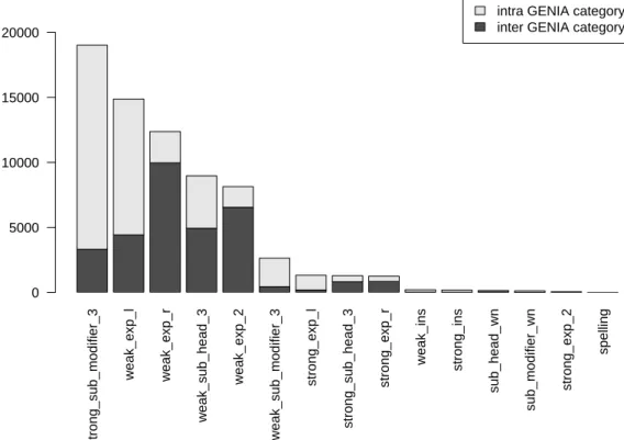
Before comparing the clustering results obtained by the different methods, we investigated the possible impact of the variations used by TermWatch on its performance. The idea was to determine if our variation relations alone could reproduce these categories, i.e., if they grouped together terms from one only GENIA class. In this case, then there would be no need to perform clustering since the variation relations alone can discover the ideal partition. However, our study showed that this was not the case.

The following chart figure (3) shows for each of our variation relation, the number of links acquired, the proportion of intra-category links and the pro-portion inter-category links (from different classes). We can see clearly from this figure that some relations are rare, i.e., they capture too few links al-though they link terms from the same class (sub modifier wn, strong ins, weak ins). These relations are in the minority especially by the proportion of terms linked. Other relations like weak exp2, weak sub head3, weak exp r are more abundant but they lead to heterogeneous clusters, they link terms from dif-ferent GENIA classes. Surprisingly, weak exp l and strong sub mod3 produced relatively good quality clusters while relating a considerable number of terms.

6.2 Evaluation of clustering results

Using the relations chosen in §5.3, CPCL on LSS generated 1, 897 non trivial components (at the COMP phase) involving only 6, 555 terms. Adding CLAS relations in the second phase led to 3, 738 clusters involving 19, 887 terms. Hierarchical clustering based on similarity matrix introduced in §5.2 generated 1, 090 clusters involving 25.129 terms for a treshold th = 0.5 and 1, 217 clusters involving 19, 867 terms for th = 0.8.

The plots in figures 4 and 5 show the results of the evaluation measures µED and µH introduced in §4.3. Since the majority of the clustering methods are sensitive to term length, we plotted the score obtained by each of the mea-sure (y-axis) by term length (x-axis). Note that at each length, only terms of that length and above are considered. For instance, at length 1, all terms are considered. At length 2, only terms having at least two words are considered. Thus, the further we move down the x-axis, the fewer the input terms for clustering.

strong_sub_modifier_3 weak_exp_l weak_exp_r weak_sub_head_3 weak_exp_2 weak_sub_modifier_3 strong_exp_l strong_sub_head_3 strong_exp_r weak_ins _{strong_ins} sub_head_wn sub_modifier_wn strong_exp_2 spelling

intra GENIA category inter GENIA category

0 5000 10000 15000 20000

Fig. 3. Distribution of related pairs of terms by variations.

Figure 4 shows the % of savings obtained by the nine algorithms tested us-ing the corrected ED measure. We see that the hierarchical method with a threshold = 0.8 and CPCL obtain a better score than the baseline clustering when considering all the terms (length ≥ 1). When fewer and longer terms are considered (length ≥ 3), partitioning methods outperform CPCL and hi-erarchical algorithms but still remain below the baseline. This is because, at length ≥ 3, CPCL has fewer terms, thus fewer relations with which to perform the clustering. Statistical methods on the other hand, with longer terms have a better context, thus more relations in the matrix. From terms of length ≥ 4 words, partitioning methods outperform the baseline.

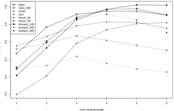
However, the ED measure masks important features of the clustering outputs since it is a compromise between the number of necessary moves and merges needed to reach the target partition. More important is the quality of the clusters (cluster homogeneity) vis-`a-vis the target partition (GENIA classes). This is measured by the µH which calculates the ratio between the value of ED and the number of movings. The µH performance of the algorithms is shown in the plot of figure 5.

1 2 3 4 5 6 −0.2 0.0 0.2 0.4 0.6 0.8

Term minimal length

Index value basic clara_300 comp cpcl hierch_05 hierch_08 kmeans_100 kmeans_300 kmeans_900

Fig. 4. Editing distance between clustering results µED and Genia categories.

significantly outperforms the baseline irrespective of term length. Hierarchical algorithm with th = 0.8 and the COMP phase of CPCL follow closely but only on all terms (length ≥ 1). Their performance drops when terms of length >= 4 are considered. Partitioning algorithms show poor cluster homogeneity. K-means with k = 100 performs worse than the other variants (Clara, k-means with k = 300, k = 900). Hierarchical with th = 0, 5 obtain the poorest score. To gain a better insight on the cluster homogeneity property, we generated for every algorithm a chart showing the proportion of terms which share the same GENIA class with the majority of terms in the same cluster (and thus that do not require any move) The nine charts are shown in figure 6.

It appears that the COMP variant of CPCL produced the most homoge-neous clusters which is not altogether surprising because the relations used in COMP phase are the most semantically tight. COMP and CPCL significantly outperform the baseline. This good performance is a bit unexpected for CPCL because the CLAS relations induce a change of head word which could lead to a semantic gap (change of semantic class).

Closely following is the hierarchical algorithm at th = 0.8. The baseline comes fourth which shows that grouping terms simply by identical head words as done

1 2 3 4 5 6 0 1 2 3 4 5

Term minimal length

Index value basic clara_300 comp cpcl hierch_05 hierch_08 kmeans_100 kmeans_300 kmeans_900

Fig. 5. Cluster homogeneity measure µED on the Genia categories.

CPCL COMP Baseline

hierch 0.8 hierch 0.5 Kmeans 100

CLARA 300 Kmeans 300 Kmeans 900

Fig. 6. Proportion of intra and inter GENIA category terms per algorithm. The black bars represent mis-classifications. White bars represent terms from the same GENIA category.

by baseline is good but not good enough to form semantically homogeneous clusters.

Partitioning methods clearly produced less homogeneous clusters. These algo-rithms showed low error rates roughly on categories with a low proportion of one word terms.

7 Concluding remarks

We have developed an efficient text mining system based on meaningful lin-guistic relations which works well on MWTs and thus on very large and sparse matrices. This method is suitable for highlighting rare phenomena which may correspond to weak signals.

The specific evaluation framework set up here led us to redefine a matrix rep-resentation in order to enable comparison with existing statistical methods. We defined a new term weighting scheme in the matrix representation en-abling statistical methods to build significant clusters. We also corrected an existing cluster evaluation measure and defined a complementary one focused on cluster homogeneity.

The choice of the evaluation metric made it possible to compare algorithms outputting very high number of clusters, with considerable differences in this number (between 100 for K-means and 3, 738 for CPCL). This was done with-out any assumption of equal cluster size. We believe these differences did not handicap any algorithm unduly since all produced clusters whose num-bers were very far from the target partition (36 classes), especially our own method. As we cannot define a priori the number of optimal clusters, CPCL’s performance was hampered for the µED measure. Statistical methods (both hierarchical and partitioning) were more sensitive to term length.

The results however show that CPCL performs well in terms of cluster qual-ity (homogenequal-ity). Since this approach is computationally tractable in linear time, it also appears to be the best candidate for tasks requiring interaction with users in real time, like interactive query refinement. This aspect will be explored in a separate study.

Overall, this experiment has shown that even without adequate context (docu-ment co-occurrence), clustering algorithms can be adapted to partially reflect a human semantic categorisation of scientific terms.

Another interesting finding of this study is that when considering an OTC or a similar task, it may be interesting to first consider clustering by a basic re-lation before resorting to more complex and fine-grained term representation. The performance of the baseline clustering in our experiment is far from poor. It could be satisfactory for some tasks, for instance as a first stage for

learn-ing new taxonomy or knowledge structures from texts. These can be further refined using more sophisticated approaches: fine-grained linguistic relations, machine learning techniques with manually tagged learning sets.

A Example of rule used in term extraction

This following simple rule translates the hypothesis that the preposition “of” plays a major role in the formation of terms. Thus prepositional phrases in-troduced by this preposition are attached to their governing NP.

From the tagged sentence:

[[The_DT inability_NN ]] of_IN [[ E1A_CD gene_NN products_NNS]] ( to_TO induce_VB ))

[[ cytolytic_JJ susceptibility_NN ]].

Our term extraction module would extract two multi-word terms (MWTs): [[ The_DT inability_NN ]] of_IN [[ E1A_CD gene_NN products_NNS]] [[ cytolytic\_JJ susceptibility\_NN ]]

This rule can be formulated as the following regular expression: If :

<mod>* <N>+ of <mod>* <N>+ <prep1> <verb> <mod>* <N>+ then return:

1) <mod>* <N>+ of <mod>* <N>+ 2) <mod>* <N>+

where:

<mod> = a determiner (DT) and/or an adjective (JJ) <N> = any of the noun tags (NN, NNS, NNPS, NNP) <prep1> = all the prepositions excluding ‘‘of’’

* = Kleene’s operator (zero or n occurrences of an item) + = at least one occurrence

B Variation rules

For the sake of clarity, all the variation rules will be given for the compound structure only.

B.0.1 Lexical variants

Modifier substitutions (sub modifier) can be identified with this simple rule:

t2 is a substitution of t1 if and only if: t1 = M m M’ h and t2 = M m’ M’ h

with m’<> m where

t1 and t2 are terms,

M and M’ are optional sequence of modifier words, m and m’ are a modifier words

h and h’ are head word.

A chain of modifier substitutions can highlight properties around the same concept. For instance, the following variants all specify a type of human cell line:

• human leukemia cell line • human lymphoblastoid cell line • human monoblastic cell line • human monocytic cell line

Head substitutions (sub head) are identified via the following rule: t2 is a substitution of t1 if and only if:

t1 = M m h and t2 = M m h’ with h’<> h

Head substitutions highlight on the other hand families of concepts sharing the same property:

• tumor cell killing • tumor cell line • tumor cell nuclei • tumor cell proliferation • tumor cell type

B.0.2 Syntactic variants

These rules identify the three types of expansion variants. • Left expansion (exp l)

t2 is a left-expansion of t1 if and only if : t1 = M h and t2 = M’ m’ M h

For example, Ad2 infection has as left expansion adenovirus 2 (Ad2) infec-tion.

• Insertion (ins)

t2 is an insertion of t1 if and only if : t1 = M1 m M2 h

t2 = M1 m m’ M’ M2 h

For instance, CD3-stimulated T lymphocyte has as insertion variant, the term CD3-stimulated human peripheral T lymphocyte. Modifier expansions enable us to create generic – specific links. Head expansions identify topical shifts as in human disease and human disease syndrome. Equivalent terms which undergo either a syntactic transformation like permutation variants (information retrieval ↔ retrieval of information) are also identified. • Right expansion (exp r)

t2 is a right-expansion of t1 if and only if : t1 = M h and t2 = M h M’ h’

An example of right expansion would be B cell development and B-cell development and differentiation. Left and right expansions (exp-2) can be combined in the same term to yield left-right expansion. An example would be the link between AIDS and second AIDS retrovirus.

References

Berry, A., Kaba, B., Nadif, M., SanJuan, E., Sigayret, A., 10-12 March 2004. Classification et d´esarticulation de graphes de termes. In: Proceedings of the 7th International conference on Textual Data Statistical Analysis (JADT 2004). Louvain-la-Neuve, Belgium, pp. 160–170.

Braam, R., Moed, H., A., A. V. R., 1991. Mapping science by combined co-citation and word analysis. 2. dynamical aspects. Journal of the American Society for Information Science 42 (2), 252–266.

Callon, T., Courtial, J., Laville, F., 1991. Co-word analysis as a tool for describ-ing the network of interactions between basic and technological research: The case of polymer chemistry. Scientometrics. 22 (1), 155–205.

Church, K. W., Hanks, P., 1990. Word association norms, mutual information and lexicography. Computational Linguistics 16 (1), 22–29.

Cutting, D., Karger, D., Pedersen, J., Tukey, O., June 21-24 1992. Scat-ter/Gather: a cluster-based approach to browsing large document collec-tions. In: 15th Annual International conference of ACM on Research and Development in Information Retrieval - ACM SIGIR. Copenhagen, Den-mark, pp. 318–329.

Denoeud, L., Garreta, H., Gu´enoche, A., May 2005. Comparison of distance indices between partitions. In: et al., P. L. (Ed.), Proceedings of Applied Stochastic Models and Data Analysis. Brest, pp. 17–20.

Docu-ment Clustering. In: Proceedings of the European Conference on Informa-tion Retrieval (ECIR’04. Sunderland, UK, pp. 167–180.

Dunning, T., 1993. Accurate methods for statistics of surprise and coincidence. Computational Linguistics (19), 61–74.

Eisen, M., Spellman, P., Brown, P., Botstein, D., 1998. Cluster analysis and display of genome-wide expression patterns. Proceedings of the National Academy of Science, USA (95), 14863–14868.

Fellbaum, C. (Ed.), 1998. WordNet, An Electronic Lexical Database. MIT Press.

Glenisson, P., Gl¨anzel, W., Janssens, F., Moor, B. D., 2005. Combining full text and bibliometric information in mapping scientific disciplines. Informa-tion Processing and Management 41 (6), 1548–1572.

Hubert, L., Arabie, P., 1985. Comparing partitions. Journal of Classification, 193–218.

Hur, B., Elisseeff, A., Guyon, I., 2002. A stability-based method for discovering structure in clustered data. Pacific Symposium on Biocomputing (7), 6–17. Ibekwe-SanJuan, F., August 1998a. A linguistic and mathematical method for mapping thematic trends from texts. In: Proceedings of the 13th European Conference on Artificial Intelligence (ECAI). Brighton, UK, pp. 170–174. Ibekwe-SanJuan, F., 10-14 August 1998b. Terminological variation, a means of

identifying research topics from texts. In: Proc. of Joint ACL-COLING’98. Qu´ebec, pp. 564–570.

Ibekwe-SanJuan, F., SanJuan, E., April 2004. Mining textual data through term variant clustering: the termwatch system. In: Proceedings of Recherche d’Information assist´ee par ordinateur (RIAO). Avignon, pp. 26–28.

Jacquemin, C., 2001. Spotting and discovering terms through Natural Lan-guage Processing. MIT Press.

Jain, A., Moreau, J., 1987. Bootstrap technique in cluster analysis. Pattern Recognition 20, 547–568.

Karypis, G., Han, E., Kumar, V., 1994. Chameleon: A hierarchical clustering algorithm using dynamic modeling. IEEE Computer: Special issue on Data analysis and mining. 32 (8), 68–75.

Kaufman, L., Rousseeuw, P., 1990. Finding Groups in Data: an Introduction to Cluster Analysis. John Wiley & Sons.

Kim, J.-D., Ohta, T., Tsuruoka, Y., Tateisi, Y., Collier, N., 2004. Introduction to the Bio-Entity Recognition Task at JNLPBA. In: In the Proceedings of JNLPBA-04. pp. 70–75.

Milligan, G. W., Cooper, M., 1985. An examination of procedures for deter-mining the number of clusters in a data set. Pychometrika 50, 159–179. Milligan, G. W., Cooper, M., 1986. A study of the comparability of external

criteria for hierarchical cluster analysis. Multivariate Behavioural Research 21, 441–458.

Ng, R., Han, J., 2002. Clarans: A method for clustering objects or spatial data mining. In: IEEE transactions on knowledge and data engineering. Vol. 14. Pantel, P., Lin, D., August 11-15 2002. Clustering by Committee. In: Annual

International conference of ACM on Research and Development in Informa-tion retrieval - ACM SIGIR. Tampere, Finland, pp. 199–206.

Polanco, X., Grivel, L., Royaut´e, J., June 7-10 1995. How to do things with terms in informetrics: terminological variation and stabilization as science watch indicators. In: Proceedings of the 5th International Conference of the International Society for Scientometrics and Informetrics. Illinois, USA, pp. 435–444.

Price, L., Thelwall, M., 2005. The clustering power of low frequency words in academic webs. Journal of the American Society for Information Science and Technology 56 (8), 883–888.

Sanjuan, E., Dowdall, J., Ibekwe-Sanjuan, F., Rinaldi, F., october 2005. A symbolic approach to automatic multiword term structering. Computer Speech Language (CSL) 19 (4), 524–542.

Smadja, F., 1993. Retrieving collocations from text: Xtract. Computational Linguistics (19), 143–177.

Tibshirani, R., Walther, G., Hastie, T., 2000. Estimating the number of clus-ters in a dataset via the gap statistic. In: Technical Report. No. 208. Dept. of Statistics, Stanford University.

Weeds, J., Dowdall, J., an B. Keller, G. S., Weir, D., 2005. Using distributional similarity to organise biomedical terminology. Terminology: Special Issue on Application-driven terminology engineering 11 (1), 107–141.

Wehrens, R., Buydens, L. M., Fraley, C., Raftery, A. E., 2003. Model-Based Clustering for Image Segmentation and Large Datasets Via Sampling. Tech. Rep. 424, Department of Statistics, University of Washington.

Yeung, K., Ruzzo, W., 2001. Details of the adjusted rand index and clustering algorithms. supplement to the paper ”an experimental study on principal component analysis for clustering gene expression data. Bioinformatics (17), 763–774.

Zitt, M., Bassecoulard, E., 1994. Development of a method for detection and trend analysis of research fronts built by lexical or co-citation analysis. Sci-entometrics. 30 (1), 333–351.