HAL Id: hal-01151695
https://hal.inria.fr/hal-01151695v2
Submitted on 22 May 2015
HAL is a multi-disciplinary open access
archive for the deposit and dissemination of
sci-entific research documents, whether they are
pub-L’archive ouverte pluridisciplinaire HAL, est
destinée au dépôt et à la diffusion de documents
scientifiques de niveau recherche, publiés ou non,
Hrishikesh Deshpande, Pierre Maurel, Christian Barillot
To cite this version:
Hrishikesh Deshpande, Pierre Maurel, Christian Barillot. Classification of Multiple Sclerosis Lesions
using Adaptive Dictionary Learning. Computerized Medical Imaging and Graphics, Elsevier, 2015,
pp.1-15. �10.1016/j.compmedimag.2015.05.003�. �hal-01151695v2�
Accepted Manuscript
Title: Classification of Multiple Sclerosis Lesions using
Adaptive Dictionary Learning
Author: Hrishikesh Deshpande Pierre Maurel Christian
Barillot
PII:
S0895-6111(15)00088-9
DOI:
http://dx.doi.org/doi:10.1016/j.compmedimag.2015.05.003
Reference:
CMIG 1376
To appear in:
Computerized Medical Imaging and Graphics
Received date:
15-1-2015
Revised date:
24-4-2015
Accepted date:
6-5-2015
Please cite this article as: Hrishikesh Deshpande, Pierre Maurel, Christian
Barillot,
Classification
of
Multiple
Sclerosis
Lesions
using
Adaptive
Dictionary Learning, Computerized Medical Imaging and Graphics (2015),
http://dx.doi.org/10.1016/j.compmedimag.2015.05.003
This is a PDF file of an unedited manuscript that has been accepted for publication.
As a service to our customers we are providing this early version of the manuscript.
The manuscript will undergo copyediting, typesetting, and review of the resulting proof
before it is published in its final form. Please note that during the production process
errors may be discovered which could affect the content, and all legal disclaimers that
apply to the journal pertain.
Accepted Manuscript
We classify multiple sclerosis lesions using adaptive dictionary learning.
Separate dictionaries are learned for the healthy brain tissues and lesion classes.
Tissue-specific information is incorporated by learning dictionaries for each tissue.
Accepted Manuscript
1 2 3 4 5 6 7 8 9 10 11 12 13 14 15 16 17 18 19 20 21 22 23 24 25 26 27 28 29 30 31 32 33 34 35 36 37 38 39 40 41 42 43 44 45 46 47 48 49 50 51 52 53 54 55 56 57Classification of Multiple Sclerosis Lesions using Adaptive
Dictionary Learning
Hrishikesh Deshpandea,b,c,d,∗, Pierre Maurela,b,c,d, Christian Barillota,b,c,d
aUniversity of Rennes 1, Faculty of Medecine, F-35043 Rennes, France bINSERM, U746, F-35042 Rennes, France
cCNRS, IRISA, UMR 6074, F-35042 Rennes, France dInria, VISAGES Project-team, F-35042 Rennes, France
Abstract
This paper presents a sparse representation and an adaptive dictionary learning based method for automated classification of Multiple Sclerosis (MS) lesions in Magnetic Res-onance (MR) images. Manual delineation of MS lesions is a time-consuming task, re-quiring neuroradiology experts to analyze huge volume of MR data. This, in addition to the high intra- and inter-observer variability necessitates the requirement of automated MS lesion classification methods. Among many image representation models and clas-sification methods that can be used for such purpose, we investigate the use of sparse modeling. In the recent years, sparse representation has evolved as a tool in modeling data using a few basis elements of an over-complete dictionary and has found applications in many image processing tasks including classification. We propose a supervised classi-fication approach by learning dictionaries specific to the lesions and individual healthy brain tissues, which include White Matter (WM), Gray Matter (GM) and Cerebrospinal Fluid (CSF). The size of the dictionaries learned for each class plays a major role in data representation but it is an even more crucial element in the case of competitive classifi-cation. Our approach adapts the size of the dictionary for each class, depending on the complexity of the underlying data. The algorithm is validated using 52 multi-sequence MR images acquired from 13 MS patients. The results demonstrate the effectiveness of our approach in MS lesion classification.
Keywords: Sparse Representations, Adaptive Dictionary Learning, Computer Aided Diagnosis, Magnetic Resonance Imaging
1. Introduction
Multiple sclerosis is a chronic, autoimmune disease of the central nervous system (CNS). It is characterized by the structural damages of axons and their myelin sheathes. Magnetic resonance imaging is the best paraclinical method for the diagnosis of MS,
∗Corresponding author
Email addresses: [email protected] (Hrishikesh Deshpande),
[email protected] (Pierre Maurel), [email protected] (Christian Barillot)
Preprint submitted to Computerized Medical Imaging and Graphics April 23, 2015 *Manuscript
Accepted Manuscript
5 6 7 8 9 10 11 12 13 14 15 16 17 18 19 20 21 22 23 24 25 26 27 28 29 30 31 32 33 34 35 36 37 38 39 40 41 42 43 44 45 46 47 48 49 50 51 52 53 54 55assessment of disease progression and treatment efficacy [1, 2]. These images are analyzed to find the number and spatial patterns of the lesions, appearance of new lesions and the total lesion load, which are key parameters in the current MS diagnostic setup. Manual segmentation of MS lesions, however, is a laborious and time consuming task, pertaining to the requirement of analyzing large number of MR images. Furthermore, it is prone to high intra- and inter-expert variability. Several MS lesion segmentation methods have been proposed over the last decades, with an objective of handling large variety of MR data and which can provide results that correlate well with expert analysis. These methods are based on supervised or unsupervised approach and use different image features and classification strategies to model lesions [3, 4].
Over the last few years, sparse representation has evolved as a model to represent an important variety of natural signals using a linear combination of a few atoms of an over-complete dictionary. Dictionary learning, a particular sparse signal model, aims at learning a non-parametric dictionary from the underlying data. The representation of data in such a manner has led to the use of sparse representations and dictionary learning in many image processing applications such as image restoration [5, 6], inpainting [7], face recognition and texture classification [8, 9].
The ability of sparse representations to approximate high-dimensional images using a few representative signals in a low-dimensional subspace and the development of effi-cient sparse coding and dictionary learning techniques offer a great advantage in medical image analysis. Recent publications have demonstrated the effectiveness of sparse repre-sentation techniques in medical applications such as shape modelling [10], constructing a structural brain network model [11] and predicting cognitive data from medical im-ages [12]. In addition, the dictionary learning framework has been used in deformable segmentation [13], image fusion [14], super-resolution analysis [15], denoising [16, 17], de-convolution of low-dose computed tomography perfusion [18, 19] and low-dose bloodbrain barrier permeability quantification [20]. In each of these applications, the dictionaries are learned from the underlying data so that they are better suited for representation of the signal of interest. On the other hand, the discriminative dictionary learning approaches proposed for image segmentation focus on learning dictionaries which are representa-tive as well as discriminarepresenta-tive [21, 22]. In this paper, we propose a novel algorithm, for classification of multiple sclerosis lesions, which incorporates discrimination in the dictionary learning framework by adjusting the size of the dictionaries according to the complexity of the underling data. Previous works [23, 24] have also reported the effects of the dictionary size in image classification. We investigate this in the particular case of classification.
In the past, Weiss et al. [25] proposed dictionary learning based MS lesion segmen-tation method by learning a single dictionary with the help of healthy brain tissue and lesion patches. The lesions are treated as outliers and lead to a higher reconstruction error when decomposed using this dictionary. There are several shortcomings in this method. The method uses only FLAIR MR images for analysis of clinical data. However, MS lesions appear in different intensity patterns in various MR sequences, which include T1-(T1-w MPRAGE), T2- (T2-w) and Proton Density-weighted (PD-w). The complemen-tary information in these MR images can further assist in classifying MS lesions. We, therefore, build our analysis using multi-channel MR data.
The former method also uses an unsupervised approach and it was observed that one of the crucial parameters used in this approach is the threshold on error map. This
Accepted Manuscript
1 2 3 4 5 6 7 8 9 10 11 12 13 14 15 16 17 18 19 20 21 22 23 24 25 26 27 28 29 30 31 32 33 34 35 36 37 38 39 40 41 42 43 44 45 46 47 48 49 50 51 52 53 54 55 56 57rameters drives the segmentation results and is not easy to tune. Furthermore, it could lead to worse segmentation results for small errors in the brain extraction procedure. We suggest a solution to this problem by proposing a fully automatic supervised classification method that eliminates this parameter. As outlined in many classification approaches using dictionary learning, we learn class specific dictionaries for the healthy brain tissues and the lesions that promote the sparse representation of the healthy and lesion patches, respectively. The lesion patches are well adapted to their own class dictionary, as op-posed to the other. Thus, we can use the reconstruction error derived from the sparse decomposition of the test patch on to these dictionaries for obtaining the classification.
There exist several MS lesion segmentation methods that use tissue segmentation to help segment the lesions [26]. We can thus further enrich our model by taking into account the tissue specific information and learning dictionaries specific to different tissue types, such as White Matter (WM), Gray Matter (GM) and Cerebrospinal Fluid (CSF), as opposed to learning a single dictionary for healthy tissue patches. We explore the fact that various tissues as well as lesions appear in different intensity patterns in distinct MR modality images. For example, WM appears as the brightest tissue in T1-weighted image, but the darkest in T2-weighted images. Therefore, learning class specific dictionaries for individual tissues should further discriminate between lesion and non-lesion classes.
The dictionaries learned for each class are aimed at better representation of an indi-vidual class. However, if there exists differences in the data-complexity between classes, the relative under- or over-representation of either class will lead to worse classification. One idea for better classification could be to learn the dictionaries with adaptive sizes, in order to take into account the data variability between different classes. Thus, in addi-tion to the dicaddi-tionary learning strategy menaddi-tioned above, we also investigate the effect of modifying the dictionary sizes, leading to the proposition of adaptive dictionary learning. The basic idea is to learn the class specific dictionaries which are better adapted to the data and also complexity of the data.
The main contributions of this paper can be outlined as follows: (1) Supervised clas-sification approach is developed using multi-channel MR data by learning dictionaries for the healthy brain tissues and the lesion classes. (2) Tissue-specific information is incorporated by learning dictionaries specific to each tissue class as opposed to learning a single dictionary for representation of the healthy brain tissue class. (3) The dictionary sizes are adapted according to the complexity of the underlying data so that the dictio-naries are better suited for representation of each class data as well as classification of MS lesions.
This paper is organized as follows. We first describe sparse coding and dictionary learning in Section 2. The materials and methods are explained in Section 3, followed by results and discussions in Section 4, and conclusion in Section 5.
2. Sparse Coding and Dictionary Learning
Sparse representation of the data allows decomposition of signals into linear combina-tion of few basis elements in the overcomplete diccombina-tionary. Consider a signal x ∈ RN and an over-complete dictionary D ∈ RN ×K. The sparse coding problem can be stated as minakak0s.t. x = Da or kx − Dak22≤ ε, where kak0is l0norm of the sparse coefficient vector a ∈ RK and ε is error in the signal representation. The efficient solvers for sparse coding include matching pursuit, orthogonal matching pursuit and basis pursuit, where
Accepted Manuscript
5 6 7 8 9 10 11 12 13 14 15 16 17 18 19 20 21 22 23 24 25 26 27 28 29 30 31 32 33 34 35 36 37 38 39 40 41 42 43 44 45 46 47 48 49 50 51 52 53 54 55the later solves the convex approximation of the problem above by replacing l0 norm with l1norm, which also results in a sparse solution [27–29]. The sparse coding problem can be given by
min
a kx − Dak 2
2+ λ kak1 (1)
where λ is called sparsity induced regularizer and balances the trade-off between the reconstruction error and the sparsity of the coefficient vector a.
The fixed dictionaries like wavelets can be efficient, but over the past years, the dictionary learning from underlying data has produced exciting results with greater data adaptability. For a set of signals {xi}i=1,.,m, the dictionary learning problem is to find D such that each signal can be represented by sparse linear combination of its atoms. This can be stated as the following optimization problem
min D,{ai}i=1,..,m m X i=1 kxi− Daik 2 2+ λ kaik1 (2)
The optimization is carried out as an iterative two-step process: (i) Sparse coding with a fixed D, and (ii) the dictionary update with a fixed a.
Among the methods available in the literature for learning the dictionary, KSVD, MOD and online dictionary learning are widely used algorithms [30–32].
3. Materials and Methods 3.1. Dataset
The proposed approach involved MR dataset of 14 MS patients acquired via Verio 3T Siemens scanner. T1-w MPRAGE, T2-w, PD-w and FLAIR modalities were chosen for the analysis. The volume size for T1-w MPRAGE and FLAIR was 256×256×160 and voxel size was 1×1×1 mm3. For T2-w and PD-w, the volume size was 256×256×44 and voxel size was 1×1×3 mm3. Annotations of the lesions were carried out on T2-w volume by an expert neuroradiologist. These manual segmentation images are referred to as ground truth lesion masks.
3.2. Overview of the method
The overview of the method proposed is shown in Figure 1. MR images for all patients are first preprocessed for noise-reduction and the elimination of extracranial brain tissues. The images are then registered into the same space. We represent image volumes as patches of a predefined size and normalize these extracted patches. This is followed by labeling patches in two ways: (i) Healthy brain tissue patches and lesion patches, using manual segmentation images and (ii) WM, GM, CSF or lesion patches, with the help of manual lesion segmentation and tissue segmentation images. The patches are then divided into the training and test dataset. For various classification strategies, we learn the dictionaries, using training data, in different configurations as follows: a single dictionary, two separate dictionaries for the healthy and lesion classes, or the class specific dictionaries for the lesions and each healthy brain tissue - WM, GM, CSF. For the last two approaches, we also study the role of the dictionary size in the classification. Finally, for a given test subject, we developed a reconstruction error based patch-classification method, which is followed by the voxel-wise classification. The following subsections briefly describe these steps.
Accepted Manuscript
1 2 3 4 5 6 7 8 9 10 11 12 13 14 15 16 17 18 19 20 21 22 23 24 25 26 27 28 29 30 31 32 33 34 35 36 37 38 39 40 41 42 43 44 45 46 47 48 49 50 51 52 53 54 55 56 57Figure 1: Flowchart of MS Lesion Classification using Dictionary Learning
3.3. Preprocessing
The noise introduced during MR acquisition is removed using non-local means and intensity inhomogenity (IIH) correction [33, 34]. To ensure the spatial correspondence, the images are registered with respect to T1-w MPRAGE volume [35] and are processed further to extract the intra-cranial mask [36]. We limit our further analysis to this brain region.
3.4. Patch extraction and labeling
For local image analysis in the dictionary learning framework, the images are divided into the overlapping patches. Each patch is then represented as a signal in the dictionary learning process. We follow this patch-based approach and divide the whole intracranial MR volume for each patient into 3-D patches, with a patch around every 2 voxels in each direction. The individual image patches of each MR modality are then flattened to form a vector and are concatenated together. The patches so obtained are normalized for a unit l1norm.
Next step is to label the normalized patches obtained from every patient. We label them in two different ways for the experiments to be preformed next. Firstly, the patches are labeled as belonging to either healthy or lesion class, using the manual segmentation image. If the number of lesion voxels in the corresponding image block of the manual
Accepted Manuscript
5 6 7 8 9 10 11 12 13 14 15 16 17 18 19 20 21 22 23 24 25 26 27 28 29 30 31 32 33 34 35 36 37 38 39 40 41 42 43 44 45 46 47 48 49 50 51 52 53 54 55segmentation image exceeds a pre-defined threshold TL, we assign this patch to the lesion class. Otherwise, it is labeled as a healthy patch. The image patches obtained in this manner form the dataset for the classification approaches which use a single dictionary or two class specific dictionaries. For other classification methods, the patches are labeled as either WM, GM, CSF or lesion class. We use the same rule, as explained above, to label the patch to the lesion class. In addition, the patch is now assigned to either WM, GM or CSF class, depending on the maximum number of voxels that belong to corresponding class in the brain tissue segmentation image obtained using Statistical Parametric Mapping (SPM) [37].
The labeled image patches are then divided into training and test data, and the exper-iments are performed by following Leave-One-Subject-Out-Cross-Validation (LOSOCV). 3.5. Patch-based classification using dictionary learning
Let n be the number of voxels per patch. For each class c, we write patches as vectors xci ∈ Rn. Learning an over-complete dictionary Dc ∈ Rn×kthat is adapted to m patches, with sparsity parameter λ, is addressed by solving the optimization problem, similar to Equation 2. min Dc,{ac i}i=1,..,m m X i=1 kxci− D c acik 2 2+ λ ka c ik1 (3)
The subsections below detail the different strategies adopted while learning these dictionaries and the scheme of patch based classification. In every method, we obtain the sparse codes for the test patches using Eq (1), knowing the dictionary Dc for the class c.
3.5.1. Single Dictionary (1D)
In the context of MS lesion classification, the simplest idea, similar to [25], could be to use a single dictionary learned from the healthy and lesion class patches. Such dictionary is mainly representative of the healthy brain image patches, based on the fact that the number of lesion patches is very small as compared to that of the healthy class. As lesions are outliers with respect to the healthy brain intensities, the decomposition of the lesion patch using such dictionary would result in a higher representation error than that for the healthy tissue patches. Thus, for a given test patch, we calculate the sparse coefficients with appropriately chosen sparse penalty factor and the reconstruction error. The test patch with representation error greater than chosen threshold would be classified as a lesion patch. For calculation of the threshold, we used the histogram of the error map, as proposed by the authors [25].
3.5.2. Two-Dictionaries: Same dictionary size (2D-S)
In this method, we learn the class specific dictionaries Dc of the same size, for the healthy (c = 1) and lesion (c = 2) class. The dictionaries learned in this manner are better suited to represent the corresponding class data. The decomposition of the test patch using other class dictionary would give rise to a higher representation error.
For a given test patch yi, the classification is performed by calculating the sparse coefficients ac
i for each class and the test patch is then assigned to the class with a
Accepted Manuscript
1 2 3 4 5 6 7 8 9 10 11 12 13 14 15 16 17 18 19 20 21 22 23 24 25 26 27 28 29 30 31 32 33 34 35 36 37 38 39 40 41 42 43 44 45 46 47 48 49 50 51 52 53 54 55 56 57minimum representation error.
cpred= argmin c
kyi− Dcacik 2
2. (4)
3.5.3. Two-Dictionaries: Different dictionary size (2D-D)
The dictionaries learned using above mentioned approach do not take into account the data variability between two classes. The size of the dictionary plays a major role in data representation. The healthy class data is associated with more variability as compared to the lesion class, because it represents complex anatomical structures such as white matter, grey matter and cerebrospinal fluid. The number of training samples for the healthy class also outnumber the lesion class training samples. To account for more variability and the number of training samples, we allow larger dictionary size for the healthy class and study its effect on MS lesion classification.
3.5.4. Four-Dictionaries: Same dictionary size (4D-S)
As explained before, the healthy brain tissues contain anatomically different regions such as WM, GM and CSF. The fact that every tissue, WM, GM and CSF, appears in different intensity pattern in each MR modality, using a single dictionary for representing the healthy brain tissues might not be as effective as learning separate dictionaries for each tissue. Adding tissue specific information in the dictionaries used for the classi-fication would enhance the prior knowledge in the learning step, thus highlighting the differences between individual tissues and also improving the lesion classification.
After learning class specific dictionaries for WM, GM, CSF and lesion, we perform classification based on reconstruction error in a similar manner, as mentioned in Sec-tion 3.5.2. Each dicSec-tionary is representative of its own class and the reconstrucSec-tion of the test data using true class dictionary would give a minimum reconstruction error. 3.5.5. Four-Dictionaries: Different dictionary size (4D-D)
Here, we experiment with different dictionary sizes for WM, GM, CSF and lesion classes, for the similar reasons mentioned in Section 3.5.3.
3.6. Voxel-wise classification
As already stated, we classify the patches centered around every 2 voxels in each direction. For voxel-wise classification, we assign each voxel to either of the classes by using majority voting. The voxel is assigned to a class using majority votes of all patches that contain the voxel.
Finally, in the context of lesion classification, we record the number of voxels that belong to True Positives (TP), False Negatives (FN) or False Positives (FP), and calculate percentage sensitivity (SEN)= T P +F NT P ×100, percentage Positive Predictive Value (PPV) =
T P ×100
T P +F P and percentage dice-score (Dice) =
2×T P ×100 2×T P +F P +F N.
4. Experiments and Results
We implemented our method using MATLAB and Python. Neuroimaging softwares N4ITK and Brain Extraction Tool (BET) were used for IIH correction and brain extrac-tion, respectively [33, 36]. The brain tissue segmentation is obtained using Statistical
Accepted Manuscript
5 6 7 8 9 10 11 12 13 14 15 16 17 18 19 20 21 22 23 24 25 26 27 28 29 30 31 32 33 34 35 36 37 38 39 40 41 42 43 44 45 46 47 48 49 50 51 52 53 54 55Pat. (a) (b) (c) (d) (e)
No. 1D 2D-S 2D-D 4D-S 4D-D
SEN PPV Dice SEN PPV Dice SEN PPV Dice SEN PPV Dice SEN PPV Dice
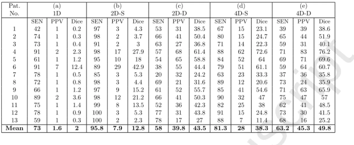
1 42 1 0.2 97 3 4.3 53 31 38.5 67 15 23.1 39 39 38.6 2 74 1 0.3 98 2 3.7 66 41 50.4 80 15 24.7 65 44 51.9 3 73 1 0.4 91 2 3 63 27 36.8 71 14 22.3 59 31 40.1 4 91 2 2.3 98 17 27.9 57 68 61.4 88 62 72.6 71 83 76.2 5 61 1 1.2 95 10 18 54 65 58.8 84 52 64 69 71 69.6 6 91 7 12.4 89 29 42.9 38 55 44.4 79 51 61.1 59 64 60.7 7 78 1 0.5 85 3 5.3 20 32 24.2 63 23 33.3 37 36 35.8 8 72 1 0.8 98 3 4.4 69 21 31.6 89 12 20.6 73 24 35.9 9 66 1 1.2 97 9 15.2 61 52 55.7 85 41 54.6 71 63 65.9 10 89 2 3.6 98 12 21.2 66 41 50.3 90 32 47 75 47 57 11 75 1 1.4 99 8 13.5 52 36 42.3 82 25 38 62 41 48.5 12 78 1 0.9 100 3 5.3 77 31 43.8 91 15 24.8 73 30 41.5 13 59 1 0.3 100 2 2.3 78 17 27 88 7 11.4 68 16 25.2 Mean 73 1.6 2 95.8 7.9 12.8 58 39.8 43.5 81.3 28 38.3 63.2 45.3 49.8
Table 1: Voxel-wise classification results using: (a) Single Dictionary, with 5000 atoms learned using the healthy and lesion class data, (b) Two class specific dictionaries with 5000 atoms each for the healthy and the lesion class, (c) 5000 atoms for the healthy and 1000 atoms for the lesion class dictionary, (d) Four class specific dictionaries with 5000 atoms each for WM, GM, CSF and the lesion classes, (e) 4000 atoms each for WM, GM and CSF classes, and 2000 atoms for the lesion class dictionary.
Parametric Mapping (SPM) [37]. The dictionary learning and sparse coding is performed with the use of SPArse Modeling Software (SPAMS) package [32].
For labeling patches, we used the threshold TL= 6, as mentioned in Section 3.5. For patch size of 5×5×5, the number of lesion patches for each patient varied from 1K to 30K, depending on the lesion load for the corresponding patient, whereas the average number of patches for the healthy brain tissue class was 1.5×10⁶. For WM, GM and CSF classes, the numbers of patches obtained per patient were 50K, 90K and 30K, respectively. The classification was performed using LOSOCV and different parameters were tested. It was found that the patch size of 5×5×5 and the sparsity parameter λ = 0.95 were optimal choices. Changing λ in steps of 0.5 from 0.5 to 0.95 did not influence the results much and the value of 0.95 provided good results for all patients. All these experiments were performed on 2.5 GHz, 120 GB RAM Xeon processor. The dictionaries of sizes ranging from 500 to 5000, were learned from the training data and the best results, in terms of both sensitivity and PPV, were selected. For the dictionary sizes varying from 500 to 5000, the dictionary learning step required 5 minutes to 3 hours, where as the classification step took 4 minutes to 38 minutes, respectively. We used these parameters for validation of classification approaches using multi-channel MR data. We, however, excluded one patient with strong MR artifacts from this analysis.
The results of voxel-wise classification, obtained using all the methods described above, are shown in Table 1. Method (a) indicates classification obtained using single dictionary learned with the help of both healthy brain tissue and lesion patches. Here, we chose the sparse penalty factor λ = 0.85 in the sparse coding step and performed the classification for various threshold values on the histogram of error map, as explained in Section 3.5.1. The threshold, which produced the best voxel-wise classification results in terms of both sensitivity and PPV, was then selected and the classification results were reported. It can be observed from very low PPV and dice-scores that this method suffers with a very large number of false positive detections.
Accepted Manuscript
1 2 3 4 5 6 7 8 9 10 11 12 13 14 15 16 17 18 19 20 21 22 23 24 25 26 27 28 29 30 31 32 33 34 35 36 37 38 39 40 41 42 43 44 45 46 47 48 49 50 51 52 53 54 55 56 57In the second experiment, we used the class specific dictionaries of same size, for the healthy and the lesion class. As indicated by method (b), the classification obtained using dictionaries with 5000 atoms each resulted in high sensitivity but PPV and dice-scores were still low. One possible reason behind these low values is that there exists a difference in variability of the data for two classes. Considering more variability associated with the healthy class data, we then used different dictionary sizes, 5000 for the healthy class and 1000 for the lesion class. As shown in method (c), this drastically reduced FP, improving PPV and dice-scores, but also decreased the sensitivity.
We further enriched this model by learning separate dictionaries for each healthy brain tissue - WM, GM, CSF, in addition to the dictionary learned for the lesion class. Using four such dictionaries with 5000 atoms each, it can be observed that a better compromise between sensitivity and PPV is achieved, as compared to methods (b) and (c) described above. This is shown by method (d). Finally, the classification using four dictionaries of different sizes, 4000 each for WM, GM and CSF classes, and 2000 for lesion class, was obtained. This reduced the mean sensitivity but improved both the mean PPV and the mean dice-score, as compared to method (d) and is indicated by method (e) in Table 1. The methods (c) and (e), which consider the inter-class data variability and use different dictionary sizes in classification, offer a better compromise between sensitivity and PPV, as compared to their counterpart methods (b) and (d), which use the same dictionary size for all classes. Between methods (c) and (e), each employing either two or four dictionaries respectively, the later method performs better than the former with a higher mean sensitivity, PPV and dice-score. Their comparison also shows a significant difference in PPV and dice-scores, with respective p-values of 0.0008 and 0.003. This confirms that the classification improves using dictionaries for each brain tissue. 4.1. Role of dictionary size on classification
To investigate the effect of dictionary size on the performance of classification, we performed the experiments using methods (d) and (e) that use three separate dictionaries for the healthy brain tissues and one for the lesion class. Table 2 summarizes the results of classification. For method (d), which uses the same dictionary size for all classes, the results along the diagonal of the table from top-left to bottom-right show that the sensitivity and PPV increase until the dictionary size is increased to 2000. The possible reason for this is that the dictionaries capture more details with the increase in their size. However, the sensitivity reduces or remains constant thereafter, possibly because of the over-fitting occurring in either class. Excluding values along the diagonal mentioned above, all other entries in the table indicate the sensitivity and PPV values obtained with method (e), which uses different dictionary sizes for tissues and the lesion class. By referring to values in the columns from a single row, which suggests using a constant dictionary size for each tissue while varying the dictionary size of lesion class from 500 to 5000, we can observe that sensitivity keeps increasing but PPV value reduces, resulting in false positive detections. On the other hand, if we fix the dictionary size for the lesion class and increase the dictionary size for the tissues, PPV increases but sensitivity reduces, resulting in under-detection. Very low PPV scores above-diagonal from top-left to bottom-right suggest that the lesion dictionary over-fits the data corresponding to the lesion class, with the use of higher dictionary size for the lesion class than that for the tissue classes. The best results, for both sensitivity and PPV together, are obtained for the dictionary size of 4000 for each tissue class and 2000 for the lesion class. It can also
Accepted Manuscript
5 6 7 8 9 10 11 12 13 14 15 16 17 18 19 20 21 22 23 24 25 26 27 28 29 30 31 32 33 34 35 36 37 38 39 40 41 42 43 44 45 46 47 48 49 50 51 52 53 54 55be observed that it is the relative dictionary size that drives the classification and is more important than just the absolute dictionary size for each class.
500 1000 2000 3000 4000 5000
SEN PPV SEN PPV SEN PPV SEN PPV SEN PPV SEN PPV
500 81.1 17.2 94.9 5.2 98.6 2.5 99.2 2.2 99.4 2.2 99.5 2.1 1000 58.3 43.7 81.8 19.7 94.5 6.8 97.2 3.9 98.0 3.0 98.5 2.6 2000 32.7 65.2 60.9 44.1 82.1 22.9 89.8 13.3 93.4 8.8 95.3 6.5 3000 19.2 72.2 46.8 56.2 71.4 36.4 82.1 25.1 87.0 18.1 90.4 13.6 4000 12.7 76.2 36.9 63.3 63.2 45.3 75.2 34.1 81.3 26.7 85.5 21.3 5000 8.9 79.5 30.0 67.5 56.9 51.1 69.2 40.5 76.2 33.4 81.3 28.0
Table 2: Effect of dictionary size in voxel-wise classification of MS lesions. The leftmost column indicates the dictionary size for each healthy tissue - WM, GM and CSF, whereas the topmost row indicates the dictionary size for the lesion class. The sensitivity and PPV values for each combination of dictionary size for the tissue and lesion classes are indicated in the corresponding entries of the table. The entries in italics on the diagonal of the table from top-left to bottom-right refer to method (d), which uses the same dictionary size for all classes, where as all other entries represent method (e) with different dictionary sizes for the tissues and the lesion class.
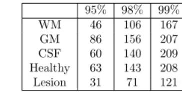
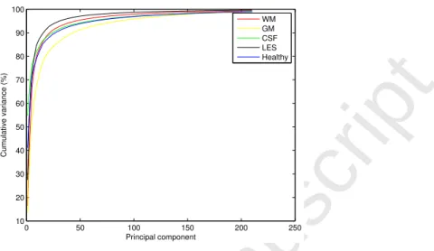
It is crucial to adapt the size of the dictionaries to better control the classification. For such purpose, we analyzed the data using Principal Component Analysis (PCA), which gives an estimate of the intrinsic dimensionality of the data. Figure 2 shows the cumulative variance explained by the eigen-vectors of different classes such as WM, GM, CSF, lesion and healthy. The number of eigen-vectors required for explaining the mentioned percentages of the total variances for each class are shown in Table 3. It can be seen that, for each brain tissue - GM, WM and CSF, approximately twice as many eigen-vectors are required for an arbitrary proportion of the percentage cumulative data variance (90%, 95% or 98%), as that required for the lesion data. As exhibited by method (e), this observation supports our adaption of dictionary size for each brain tissue twice that for the lesion dictionary. In case of method (c), which uses dictionaries for healthy and lesion classes, the experimentally observed optimal dictionary size ratio of 5 for the healthy and the lesion class was not found with PCA. Although, the factor 2 indicated by PCA still favors using a higher dictionary size for the healthy class. One reasoning behind this failure might be the inability of PCA to analyze the non-linearity in the data. The intrinsic dimensionality estimation for this highly non-linear data could be further point of investigation. 95% 98% 99% WM 46 106 167 GM 86 156 207 CSF 60 140 209 Healthy 63 143 208 Lesion 31 71 121
Table 3: Principal component analysis of the training data for an arbitrarily selected patient. For each class mentioned in a row, an entry in the table denotes the number of eigen-vectors required to attain the percentage of total variance indicated in each column.
Accepted Manuscript
1 2 3 4 5 6 7 8 9 10 11 12 13 14 15 16 17 18 19 20 21 22 23 24 25 26 27 28 29 30 31 32 33 34 35 36 37 38 39 40 41 42 43 44 45 46 47 48 49 50 51 52 53 54 55 56 57 0 50 100 150 200 250 10 20 30 40 50 60 70 80 90 100 Principal component Cumulative variance (%) WM GM CSF LES HealthyFigure 2: Cumulative variance for different classes, plotted against the number of principal components obtained from the principle component analysis of the corresponding class data.
4.2. Extending the training database
We are aware that we do not have a very large population for training. To investigate if the size of the training data has any effect on the classification results, we incorporated longitudinal database into our analysis. MR volumes are acquired for each patient, at time points M0, M3 and M6, with an interval of three months. As the lesions evolve over the course of time, some lesions might disappear partially or fully, and there might be some newly appearing lesions. It is therefore fair to consider that each dataset at consecutive time point would result in adding different lesion patterns in the training procedure. Thus, we modified the training data, for each patient, in two ways: (1) Data at time-points M0 and M3, with 24 datasets and (2) Data at time-points M0, M3 and M6, with 36 datasets. However, the lesion classification experiments for the same test subjects, as in previous experiments, using class specific dictionaries with 5000 and 1000 atoms for the healthy and lesion class respectively, did not show any significant improvement in the sensitivity and PPV. This suggests that the size of the population for training the dictionaries is not a critical issue for such approaches.
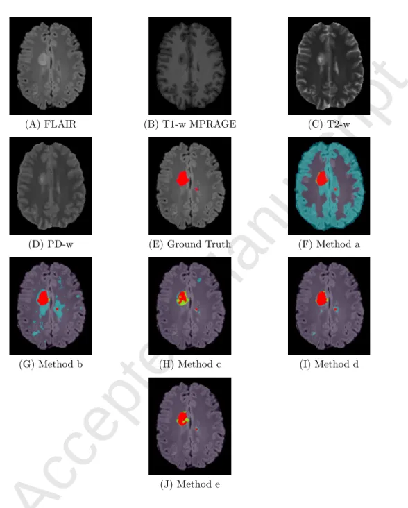
In Figures 3 and 4, we show the voxel-wise classification results obtained using all methods discussed above. We arbitrarily selected a slice for the patients 4 and 6, as referred to in Table 1. It can be seen from Figure 3F that method (a) suffers with a large number of FP. The over-detections are reduced in methods (b) and (d), which use dictionaries of the same size for each class. This is indicated in Figures 3G and 3I, respectively. Methods (c) and (e) further improve the classification, as shown in Figures 3H and 3J, by employing the dictionaries of adapted sizes. However, the 2-class method (c) has many FN. As shown by method (e), including tissue specific information in such adaptive dictionary learning based approach results in significant improvement in the lesion classification with reduction in both FP and FN. This supports our claim that the method with the tissue specific dictionaries and adapted dictionary sizes is a better choice over the 2-class methods and those using the same dictionary size for all classes.
Accepted Manuscript
5 6 7 8 9 10 11 12 13 14 15 16 17 18 19 20 21 22 23 24 25 26 27 28 29 30 31 32 33 34 35 36 37 38 39 40 41 42 43 44 45 46 47 48 49 50 51 52 53 54 55(A) FLAIR (B) T1-w MPRAGE (C) T2-w
(D) PD-w (E) Ground Truth (F) Method a
(G) Method b (H) Method c (I) Method d
(J) Method e
Figure 3: Comparison of MS lesion classification methods, example 1 - patient 6, slice 164. (A) FLAIR, (B) T1-w MPRAGE, (C) T2-w, (D) PD-w, (E) Ground truth or manual lesion segmentation image (shown in red) superimposed on FLAIR, (F) Result for method (a) using single dictionary with 5000 atoms learned using the healthy and lesion class data, (G) Result for method (b) with two dictionaries containing 5000 atoms each for the healthy and the lesion class, (H) Result for method (c) with 5000 atoms for the healthy and 1000 atoms for the lesion class dictionary, (I) Result for method (d) with four class specific dictionaries with 5000 atoms each for WM, GM, CSF and the lesion classes, (J) Result for method (e) with 4000 atoms each for WM, GM and CSF class, and 2000 atoms for the lesion class dictionary. Classification image is overlayed on FLAIR MRI. Red: TP; Cyan: FP; Green: FN.
Accepted Manuscript
1 2 3 4 5 6 7 8 9 10 11 12 13 14 15 16 17 18 19 20 21 22 23 24 25 26 27 28 29 30 31 32 33 34 35 36 37 38 39 40 41 42 43 44 45 46 47 48 49 50 51 52 53 54 55 56 57(A) FLAIR (B) T1-w MPRAGE (C) T2-w
(D) PD-w (E) Ground Truth (F) Method a
(G) Method b (H) Method c (I) Method d
(J) Method e
Figure 4: Comparison of MS lesion classification methods, example 2 - patient 4, slice 153. (A) FLAIR, (B) T1-w MPRAGE, (C) T2-w, (D) PD-w, (E) Ground truth or manual lesion segmentation image (shown in red) superimposed on FLAIR, (F)-(J) Results of voxel-wise classification obtained using meth-ods (a)-(e), as mentioned in Figure 3. Classification image is overlayed on FLAIR MRI. Red: TP; Cyan: FP; Green: FN.
Accepted Manuscript
5 6 7 8 9 10 11 12 13 14 15 16 17 18 19 20 21 22 23 24 25 26 27 28 29 30 31 32 33 34 35 36 37 38 39 40 41 42 43 44 45 46 47 48 49 50 51 52 53 54 55 5. ConclusionTo automatically classify multiple sclerosis lesions, we proposed a novel supervised approach using sparse representations and dictionary learning. The methods using class specific dictionaries outperform the classification obtained using a single dictionary, in which the lesions are modeled as outliers. Learning more specific dictionaries for each anatomical structure in the brain helps improve the classification on account of specific intensity patterns associated with each of these structures in multi-channel MR images. We have also demonstrated the effectiveness of adapting the dictionary sizes for better amplification of differences among multiple classes, hence improving the classification. If performing PCA on input data can successfully adapt the dictionary size for the classification, it is not as much efficient when the classes represent more a mixture of different tissues. Knowing the limitation of PCA to handle only linear data, future work will be to use the intrinsic dimension estimation techniques, which can better analyze complexity of the non-linear data.
References
[1] R. Grossman, J. McGowan, Perspectives on multiple sclerosis, American journal of neuroradiology 19 (7) (1998) 1251–1265.
[2] D. H. Miller, M. Filippi, F. Fazekas, J. L. Frederiksen, P. M. Matthews, X. Montalban, C. H. Polman, Role of magnetic resonance imaging within diagnostic criteria for multiple sclerosis, Annals of Neurology 56 (2) (2004) 273–278.
[3] D. Garc´ıa-Lorenzo, S. Francis, S. Narayanan, D. L. Arnold, D. L. Collins, Review of automatic segmentation methods of multiple sclerosis white matter lesions on conventional magnetic resonance imaging, Medical Image Analysis 17 (1) (2013) 1 – 18.
[4] X. Llad´o, A. Oliver, M. Cabezas, J. Freixenet, J. C. Vilanova, A. Quiles, L. Valls, L. Rami-Torrent, lex Rovira, Segmentation of multiple sclerosis lesions in brain MRI: A review of automated ap-proaches, Information Sciences 186 (1) (2012) 164 – 185.
[5] M. Elad, M. Aharon, Image denoising via learned dictionaries and sparse representation, in: IEEE Computer Society Conference on Computer Vision and Pattern Recognition, Vol. 1, 2006, pp. 895–900.
[6] J. Mairal, M. Elad, G. Sapiro, Sparse representation for color image restoration, IEEE Transactions on Image Processing 17 (1) (2008) 53–69.
[7] M. Elad, M. Figueiredo, Y. Ma, On the role of sparse and redundant representations in image processing, Proceedings of the IEEE 98 (6) (2010) 972–982.
[8] G. Peyr´e, Sparse modeling of textures, Journal of Mathematical Imaging and Vision 34 (1) (2009) 17–31.
[9] J. Wright, A. Yang, A. Ganesh, S. Sastry, Y. Ma, Robust face recognition via sparse representation, IEEE Transactions on Pattern Analysis and Machine Intelligence 31 (2) (2009) 210–227.
[10] S. Zhang, Y. Zhan, M. Dewan, J. Huang, D. N. Metaxas, X. S. Zhou, Towards robust and effective shape modeling: Sparse shape composition, Medical Image Analysis 16 (1) (2012) 265 – 277. [11] M. Chung, H. Lee, P. Kim, J. C. Ye, Sparse topological data recovery in medical images, in: IEEE
International Symposium on Biomedical Imaging: From Nano to Macro, 2011, pp. 1125–1129. [12] B. Kandel, D. Wolk, J. Gee, B. Avants, Predicting cognitive data from medical images using sparse
linear regression, in: Information Processing in Medical Imaging, Vol. 7917 of Lecture Notes in Computer Science, Springer Berlin Heidelberg, 2013, pp. 86–97.
[13] S. Zhang, Y. Zhan, D. N. Metaxas, Deformable segmentation via sparse representation and dic-tionary learning, Medical Image Analysis 16 (7) (2012) 1385 – 1396, special Issue on the 2011 Conference on Medical Image Computing and Computer Assisted Intervention.
[14] N.-N. Yu, T.-S. Qiu, W.-h. Liu, Medical image fusion based on sparse representation with ksvd, in: M. Long (Ed.), World Congress on Medical Physics and Biomedical Engineering May 26-31, 2012, Beijing, China, Vol. 39 of IFMBE Proceedings, Springer Berlin Heidelberg, 2013, pp. 550–553.
Accepted Manuscript
1 2 3 4 5 6 7 8 9 10 11 12 13 14 15 16 17 18 19 20 21 22 23 24 25 26 27 28 29 30 31 32 33 34 35 36 37 38 39 40 41 42 43 44 45 46 47 48 49 50 51 52 53 54 55 56 57[15] Y.-H. Wang, J.-B. Li, P. Fu, Medical image super-resolution analysis with sparse representation, in: Eighth International Conference on Intelligent Information Hiding and Multimedia Signal Pro-cessing (IIH-MSP), 2012, pp. 106–109.
[16] R. Rubinstein, M. Zibulevsky, M. Elad, Double sparsity: Learning sparse dictionaries for sparse signal approximation, IEEE Transactions on Signal Processing 58 (3) (2010) 1553–1564.
[17] B. Deka, P. Bora, Despeckling of medical ultrasound images using sparse representation, in: Inter-national Conference on Signal Processing and Communications (SPCOM), 2010, pp. 1–5. [18] R. Fang, T. Chen, P. C. Sanelli, Tissue-specific sparse deconvolution for low-dose ct perfusion,
Inter-national Conference on Medical Image Computing and Computer-Assisted Intervention (MICCAI) 16 (Pt 1) (2013) 114121.
[19] R. Fang, T. Chen, P. C. Sanelli, Towards robust deconvolution of low-dose perfusion ct: Sparse perfusion deconvolution using online dictionary learning, Medical Image Analysis 17 (4) (2013) 417 – 428.
[20] R. Fang, K. Karlsson, T. Chen, P. C. Sanelli, Improving low-dose bloodbrain barrier permeability quantification using sparse high-dose induced prior for patlak model, Medical Image Analysis 18 (6) (2014) 866 – 880, sparse Methods for Signal Reconstruction and Medical Image Analysis.
[21] S. Zhang, J. Huang, D. Metaxas, W. Wang, X. Huang, Discriminative sparse representations for cervigram image segmentation, in: IEEE International Symposium on Biomedical Imaging: From Nano to Macro, 2010, pp. 133–136.
[22] T. Tong, R. Wolz, P. Coup, J. V. Hajnal, D. Rueckert, Segmentation of MR images via discrim-inative dictionary learning and sparse coding: Application to hippocampus labeling, NeuroImage 76 (0) (2013) 11 – 23.
[23] H. Deshpande, P. Maurel, C. Barillot, Detection of multiple sclerosis lesions using sparse represen-tations and dictionary learning, in: MICCAI workshop on Sparsity Techniques in Medical Imaging, 2014, pp. 71–79.
[24] I. Ramirez, G. Sapiro, An MDL framework for sparse coding and dictionary learning, IEEE Trans-actions on Signal Processing 60 (6) (2012) 2913–2927.
[25] N. Weiss, D. Rueckert, A. Rao, Multiple sclerosis lesion segmentation using dictionary learning and sparse coding, in: Medical Image Computing and Computer-Assisted Intervention MICCAI 2013, Vol. 8149, 2013, pp. 735–742.
[26] A. Zijdenbos, R. Forghani, A. Evans, Automatic ”pipeline” analysis of 3-D MRI data for clinical trials: application to multiple sclerosis, IEEE Transactions on Medical Imaging 21 (10) (2002) 1280–1291.
[27] S. Mallat, Z. Zhang, Matching pursuits with time-frequency dictionaries, IEEE Transactions on Signal Processing 41 (12) (1993) 3397–3415.
[28] Y. Pati, R. Rezaiifar, P. Krishnaprasad, Orthogonal matching pursuit: recursive function approxi-mation with applications to wavelet decomposition, in: 1993 Conference Record of the 27th Asilomar Conference on Signals, Systems and Computers, 1993, pp. 40–44 vol.1.
[29] S. S. Chen, D. L. Donoho, Michael, A. Saunders, Atomic decomposition by basis pursuit, SIAM Journal on Scientific Computing 20 (1998) 33–61.
[30] M. Aharon, M. Elad, A. Bruckstein, K -SVD: An algorithm for designing overcomplete dictionaries for sparse representation, IEEE Transactions on Signal Processing 54 (11) (2006) 4311–4322. [31] K. Engan, S. Aase, J. Husoy, Frame based signal compression using method of optimal directions
(MOD), in: IEEE International Symposium on Circuits and Systems, Vol. 4, 1999, pp. 1–4 vol.4. [32] J. Mairal, F. Bach, J. Ponce, G. Sapiro, Online dictionary learning for sparse coding, in: Proceedings
of International Conference on Machine Learning, 2009.
[33] N. Tustison, B. Avants, P. Cook, Y. Zheng, A. Egan, P. Yushkevich, J. Gee, N4ITK: Improved N3 bias correction, IEEE Transactions on Medical Imaging 29 (6) (2010) 1310–1320.
[34] P. Coupe, P. Yger, S. Prima, P. Hellier, C. Kervrann, C. Barillot, Optimized blockwise nonlocal means denoising filter for 3-D magnetic resonance images, IEEE Transactions on Medical Imaging 27 (4) (2008) 425–441.
[35] W. Wells, P. Viola, H. Atsumi, S. Nakajima, R. Kikinis, Multi-modal volume registration by max-imization of mutual information, Medical Image Analysis 1 (1) (1996) 35 – 51.
[36] S. Smith, Fast robust automated brain extraction, Human Brain Mapping 17 (3) (2002) 143–155. [37] J. Ashburner, K. Friston, Unified segmentation, NeuroImage 26 (3) (2005) 839 – 851.