Elasto-plastic analysis of bonded joints with macro-elements

HAL Id: hal-00926995

https://hal.archives-ouvertes.fr/hal-00926995

Submitted on 10 Jan 2014

HAL is a multi-disciplinary open access

archive for the deposit and dissemination of

sci-entific research documents, whether they are

pub-lished or not. The documents may come from

teaching and research institutions in France or

abroad, or from public or private research centers.

L’archive ouverte pluridisciplinaire HAL, est

destinée au dépôt et à la diffusion de documents

scientifiques de niveau recherche, publiés ou non,

émanant des établissements d’enseignement et de

recherche français ou étrangers, des laboratoires

publics ou privés.

Elasto-plastic analysis of bonded joints with

macro-elements

Eric Paroissien, Fréderic Gaubert, A. da Veiga, Frederic Lachaud

To cite this version:

Eric Paroissien, Fréderic Gaubert, A. da Veiga, Frederic Lachaud. Elasto-plastic analysis of bonded

joints with macro-elements. Journal of Adhesion Science and Technology, Taylor & Francis, 2013, vol.

27, pp. 1464-1498. �10.1080/01694243.2012.745053�. �hal-00926995�

This is an author-deposited version published in:

http://oatao.univ-toulouse.fr/

Eprints ID: 9309

To link to this article: DOI: 10.1080/01694243.2012.745053

URL:

http://dx.doi.org/10.1080/01694243.2012.745053

To cite this version:

Paroissien, Eric and Gaubert, Fréderic and Da Veiga,

A. and Lachaud, Frédéric Elasto-plastic analysis of bonded joints with

macro-elements. (2013) Journal of Adhesion Science and Technology, vol.

27 (n° 13). pp. 1464-1498. ISSN 0169-4243

O

pen

A

rchive

T

oulouse

A

rchive

O

uverte (

OATAO

)

OATAO is an open access repository that collects the work of Toulouse researchers and

makes it freely available over the web where possible.

Any correspondence concerning this service should be sent to the repository

administrator:

staff-oatao@inp-toulouse.fr

Elasto-plastic analysis of bonded joints

with macro-elements

E. Paroissien a , F. Gaubert a , A. Da Veiga a & F. Lachaud b a

Sogeti High Tech, Parc le Millénaire – Bât A1, Avenue de l’Escadrille Normandie Niemen, Blagnac, 31700, France b

Institut Clément Ader, ISAE/DMSM, Campus ENSICA, 1 Place Emile Blouin, Toulouse, 31500, France

Elasto-plastic analysis of bonded joints with macro-elements

E. Paroissiena,*, F. Gauberta, A. Da Veigaaand F. Lachaudb

a

Sogeti High Tech, Parc le Millénaire – Bât A1, Avenue de l’Escadrille Normandie Niemen, Blagnac

31700, France;bInstitut Clément Ader, ISAE/DMSM, Campus ENSICA, 1 Place Emile Blouin, Toulouse

31500, France

The Finite Element (FE) method could be able to address the stress analysis of bonded joints. Nevertheless, analyses based on FE models are mainly computationally cost expen-sive and it would be profitable to develop simplified approaches, enabling extenexpen-sive para-metric studies. Firstly, a one-dimensional 1D-bar and 1D-beam simplified models for the bonded joint stress analysis, assuming a linear elastic adhesive material, are presented. These models derive from an approach, inspired by the FE method using a formulation based on a four-node macro-element, which is able to simulate an entire bonded overlap. Moreover, a linear shear stress variation in the adherend thickness is included in the formu-lation. Secondly, a numerical procedure is then presented to introduce into both models an elasto-plastic adhesive material behavior, while keeping the previous linear elastic formula-tion. Finally, assuming an elastic perfectly plastic adhesive material behavior, the results produced by simplified models are compared with the results predicted by FE using 1D-bar, plane stress, and three-dimensional (3D) models. Good agreements are shown. Keywords: bonded joint; single-lap shear; nonlinear material adhesive; Finite Element method; analytical formulation; macro-element

1. Introduction

1.1. Context

In the frame of the structural component design, bonding can be considered as a suitable assembly method or an attractive complement to conventional methods such as bolting or riv-eting. Bonding offers the possibility of joining without damaging various materials, like plas-tics or metals, as well as allowing for various combinations of materials. This first advantage is reinforced by a large choice of adhesive families and by the possibility to formulate adhe-sives, designed to best meet the joint specifications, while optimizing the structure. Bonding allows mainly for mass benefits with regard to other mechanical fastening methods, since the material volume required is reduced to sustain static or fatigue loads. The Finite Element (FE) method could be able to address the stress analysis of bonded joints. Nevertheless, anal-yses based on FE models are mainly computationally cost expensive and it would be profit-able to develop simplified approaches, enabling extensive parametric studies. The study, presented in this paper, takes place in this context. As highlighted in several literature surveys *Corresponding author. Email: eric.paroissien@sogeti.com

[1–3], a large number of simplified approaches for the stress analysis of bonded joints exist in the open literature.

1.2. Objective

The objective of this paper is to present a simplified approach for the stress analysis of bonded joints, taking into account an elasto-plastic adhesive material behavior. This topic was already addressed by several authors (e.g. [4–11]) leading to the presentation of semi-analyti-cal solutions. Indeed, in order to enlarge the application field of models, the number of sim-plifying hypotheses has to be restricted. The resolution of the complete set of governing equations, derived from the restricted hypotheses, requires then the development of dedicated procedures, even under the assumption of linear elastic material behaviors. In this paper, a restricted number of simplifying hypotheses is similarly under consideration, so that closed-form solutions are not provided. However, an original procedure allowing for the resolution is presented. The simplified approach, presented in this paper, consists then in an iterative res-olution scheme, using a simplified linear elastic method for the stress analysis of bonded joints. The simplified linear elastic method is based on the analytical formulation of a four-node macro-element, in the frame of both one-dimensional 1D-bar and 1D-beam analyses. It is then exemplified on the single-lap bonded joint configuration (see Figure 1 and Table 1).

1.3. Overview of the simplified linear elastic method

The simplified linear elastic method, originally presented in [12,13], is inspired by the FE method and allows for the resolution of the set of governing differential equations. The dis-placements and forces in the adherends as well as the adhesive stresses are then computed. The method consists in meshing the structure in elements. A full bonded overlap is meshed by a unique four-node macro-element, which is specially formulated. This macro-element is called bonded-bars (BBa) or bonded-beams (BBe), depending on the 1D-analysis frame. According to the classical FE rules, the stiffness matrix of the structure – termed K – is

Figure 1. Idealization of a single-lap bonded joint with beam and BBe elements, for example. The

assembled and the selected boundary conditions are applied. The minimization of the total potential energy leads to find the vector of nodal displacements U such that F = KU, where F is the vector of nodal forces. This approach based on macro-elements takes advantage of the flexibility of FE method. Indeed, by employing a macro-element as an elementary brick, it offers the possibility to simulate complex structures involving single-lap bonded joints [14]. Only simple manipulations on the stiffness matrix of the structure are required. An approach for the simulation of hybrid (bolted/bonded) joints can consist in employing macro-elements for the bonded parts and springs for the fasteners [12,13]. Finally, various mechanical or thermal loadings could be taken into account, through the vector of nodal forces.

1.4. Overview of the paper

The mechanical and geometrical parameters are free; in particular, unbalanced configurations can be addressed. In the 1D-bar (1D-beam) frame, the adherends are simulated as linear elas-tic bars (as laminated linear elaselas-tic Euler–Bernoulli beams), while the adhesive layer simula-tion consists in continuously distributed linear or nonlinear shear springs (in continuously distributed linear or nonlinear shear and peeling springs). The adhesive layer thickness is assumed to be constant along the overlap.

BBa and BBe elements were previously developed [12,13,15]. Nevertheless, they do not take into account the shear stress in the adherends. The first part of the paper is then dedi-cated to the detailed presentation of the formulation of 1D-bar and 1D-beam macro-elements, including a linear variation of shear stress in the adherends, according to the approach of Tsai and Morton [16]. Elements of validation are presented, by showing that under the same hypotheses as the Tsai and Morton model, the same results are obtained. Secondly, the intro-duction of an iterative resolution scheme is presented, to take into account an elasto-plastic adhesive material behavior. The projection algorithm with elastic matrix is employed for the numerical resolution. Thirdly, a 1D-bar FE model, involving bar elements and shear springs, is developed as a numerical image of the simplified 1D-bar model. Besides, a plane stress (PS) and three-dimensional (3D) FE models are developed to assess the performances of the simplified 1D-beam model.

2. Linear elastic 1D-bar and 1D-beam models

2.1. 1D-bar model

2.1.1. Formulation of the BBa element

2.1.1.1. Hypotheses. The model is based on the following hypotheses: (i) the thickness of the adhesive layer is constant along the overlap, (ii) the adherends are linear elastic materials simulated as bars, (iii) the adhesive layer is simulated by an infinite number of linear elastic shear springs linking both adherends, and possibly (iv) the adherend shear stress varies line-arly with the adherend thickness.

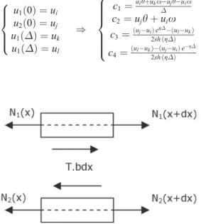
2.1.1.2. Governing equations. The local equilibrium of both adherends (see Figure 2) and the linear elastic material behavior provide the following set of governing equations:

Table 1. Geometrical and mechanical parameters of the nominal single-lap joint under consideration.

b (mm) e (mm) e1= e2(mm) L (mm) l1= l2(mm) E (MPa) E1= E2(MPa) ν ν1= ν2

dNj dx ¼ ð#1Þ j bT Nj¼ Ejbej duj dx; j¼ 1; 2 T ¼ Gu2#u1 e 8 > < > : ð1Þ

where, e is the adhesive thickness, e1 (e2) is the thickness of the adherend 1 (2), b is the

width, G is the adhesive shear modulus, E1 (E2) is the Young’s modulus of the adherend 1

(2), N1(N2) is the normal force in the adherend 1 (2), and T is the adhesive shear stress. The

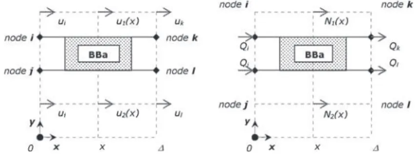
displacements u1(x) (u2(x)) are the normal displacements of points located at the abscissa x

on the neutral line of adherend 1 (2) before deformation (see Figure 3).

2.2.1.3. Stiffness matrix of the BBa element. The system of Equation (1) leads to the follow-ing system of linear differential equations:

d2_u 1 dx2 þ G eE1e1ðu2# u1Þ ¼ 0 d2_u 1 dx2 þ G eE2e2ðu2# u1Þ ¼ 0 ( ð2Þ The system of Equation (2) is solved as:

u1¼ 0:5 ½#h ðc3e#gxþ c4egxÞ þ c1xþ c2' u2¼ 0:5 ½x ðc3e#gxþ c4egxÞ þ c1xþ c2' & with: h_{¼ 1 þg}w2 x_{¼ 1 #g}w2 w¼G e ð 1 e1E1# 1 e2E2Þ g2_¼G e ð 1 e2E2þ 1 e1E1Þ 8 > > > < > > > : ð3Þ

where, c1, c2, c3, and c4are the integration constants.

The boundary conditions at both extremities of the BBa element, in terms of displace-ments, lead to expressions for the integration constants, as functions of nodal displacements ui, uj, uk, and ul(see Figure 3):

u1ð0Þ ¼ ui u2ð0Þ ¼ uj u1ð!Þ ¼ uk u1ð!Þ ¼ ul ) 8 > > < > > : c1¼ ulhþukx#ujh#uix ! c2¼ ujhþ uix c3¼ðuj#uiÞ e g!_#ðu l#ukÞ 2shðg!Þ c4¼ðul#ukÞ#ðuj#uiÞ e #g! 2shðg!Þ 8 > > > > < > > > > : ð4Þ

where, Δ is the length of the BBa element.

The linear elastic behavior of adherends allows then for the expression of adherend nor-mal forces as a function of nodal displacements, through the integration constants (Equations (1) and (3)):

N1¼ 0:5 b E1e1½hgðc1e#gx# c2egxÞ þ c3'

N2¼ 0:5 b E2e2½xgðc2egx# c1e#gxÞ þ c3'

&

ð5Þ In the same way, the adhesive shear stress is then computed with Equation (3) as:

T ¼ 0:5 b E1e1bhg ðc1e#gx# c2egxÞ þ c3c ð6Þ

The nodal forces Qi, Qj, Qk, and Ql, which represent the action of nodes i, j, k, and l,

respectively on the BBa element (see Figure 3) can be expressed as functions of nodal displacements (Equation (5)): Qi¼ #N1ð0Þ Qj¼ #N2ð0Þ Qk ¼ N1ð!Þ Ql¼ N2ð!Þ ) Qi¼ #0:5 b E1e1½hg ðc1# c2Þ þ c3' Qj¼ #0:5 b E2e2½xg ðc2# c1Þ þ c3' Qk¼ 0:5 b E1e1½hg ðc1e#g!# c2eg!Þ þ c3' Ql¼ 0:5 b E2e2½xg ðc2eg!# c1e#g!Þ þ c3' 8 > > > > < > > > > : 8 > > > > < > > > > : ð7Þ

The stiffness matrix of the BBa element is defined by: kii kij kik kil kji kjj kjk kjl kki kkj kkk kkl kli klj klk kll 2 6 6 6 4 3 7 7 7 5 ui uj uk ul 2 6 6 6 4 3 7 7 7 5 ¼ Qi Qj Qk Ql 2 6 6 6 4 3 7 7 7 5 ð8Þ where, krs¼ @Qr @us ; r; s¼ i; j; k; l ð9Þ

Finally, the stiffness matrix of the BBa element, named KBBa, can be written as:

KBBa¼ x E2e2b 2! g! thðg!Þþ E1e1 E2e2 1# g! thðg!Þ # g! shðg!Þ# E1e1 E2e2 g! shðg!Þ# 1 1# g! thðg!Þ g! thðg!Þþ E2e2 E1e1 g! shðg!Þ# 1 # g! shðg!Þ# E2e2 E1e1 # g! shðg!Þ# E1e1 E2e2 g! shðg!Þ# 1 g! thðg!Þþ E1e1 E2e2 1# g! thðg!Þ g! shðg!Þ# 1 # g! shðg!Þ# E2e2 E1e1 1# g! thðg!Þ g! thðg!Þþ E2e2 E1e1 0 B B B B @ 1 C C C C A ð10Þ

2.1.1.4. Considering the shear stress in the adherends. Following [16], a linear distribution of the shear stress, named T1(T2), in the thickness of the adherend 1 (2) is assumed:

Tj¼ # T 2 1þ ð#1Þ j 2yj ej 3 4 ; j¼ 1; 2 ð11Þ

where, y1and y2are local y-axes, as defined in Figure 1.

The shear deformation, named γ1(γ2), in the adherend 1 (2) is then given by:

cj¼ Tj Gj¼ # 1 2 1þ ð#1Þ j 2yj ej 3 _{4 T} Gj¼ @ujðx; yjÞ @yj ; j¼ 1; 2 ð12Þ

where, G1(G2) is the shear modulus of the adherend 1 (2).

The integration of Equation (12) allows for the expression of the normal displacements of adherends, as functions of x and yj:

ujðx; yjÞ ¼ u1ðx; 0Þ þ Z yj 0 Tj Gj dyj ) u1ðx; y1Þ ¼ u1ðx; 0Þ þ_2GT₁ y2 1 e1# y1 6 7 u2ðx; y2Þ ¼ u2ðx; 0Þ #_2GT₂ y2 2 e2þ y2 6 7 8 < : ð13Þ The normal forces in the adherends are then deduced:

Nj¼ b Z ej₂ #ej2 Ej @ujðx; yjÞ @x dyj ) N1¼ be1E1 du1ðx;0Þ dx # 1 3 e1 G2 dT dx 6 7 N2¼ be2E2 du2ðx;0Þ dx þ 1 3 e1 G2 dT dx 6 7 8 < : ð14Þ But, by noticing that the average value of the normal displacement on the adherend thick-ness is given by:

" uj¼ 1 ej Z ej₂ #ej2 ujðx; yjÞ dyj ) " u1¼ u1ðx; 0Þ #1₃e1_GT₁ " u2¼ u2ðx; 0Þ þ1₃e2_GT₂ ( ð15Þ

the normal forces in the adherends and the adhesive shear stress can be written as: Nj¼ bejEj d"uj dx T ¼ "G"u2#"u1 e & with " G¼ G 1þn2 n2_¼1 3 G eð e1 G1þ e2 G2Þ ( ð16Þ Finally, to take into account a linear variation of the shear stress in the adherends, the res-olution consists in substituting G by "G and uj by "uj, in the formulation, which does not

2.1.2. Assembly and validation on the exemplified single-lap joint

The single-lap bonded joint is meshed as following: (i) the overlap is meshed which 1 BBa element, (ii) each adherend outside the overlap is meshed with 1 bar element. This mesh leads to a total number of six nodes (see Figure 4).

The stiffness matrix of the single-lap joint is then assembled, according to the classical FE rules, through the stiffness matrices of each element. The stiffness matrix for the bar ele-ment, named Kbar, is:

Kbar ¼ Ejejb lj 1 #1 #1 1 3 4 ; j¼ 1; 2 ð17Þ

where, l1(l2) is the length of the bar outside the overlap of the adherend 1 (2).

Following the classical FE rules, the boundary conditions are then applied to the single-lap bonded joint, which is clamped at one extremity and free to move at the other one, where a force f = 10 N is applied (see Figure 4). A total number of degrees of freedom (DoF) equal to 5 is then involved. The resolution consists then in inverting a 5+ 5 linear system.

The adhesive stress distribution predicted by [16] is compared to the model predictions for the single-lap bonded joint defined in Figure 1 and Table 1. The superimposition of curves shown in Figure 5 allows for the conclusion that the same hypotheses lead to the same results.

2.2. 1D-beam model

2.2.1. Formulation of the BBe element

2.2.1.1. Hypotheses. The model is based on the following hypotheses: (i) the thickness of the adhesive layer is constant along the overlap, (ii) the adherends are simulated by linear elastic Euler–Bernoulli laminated beams, (iii) the adhesive layer is simulated by an infinite number of elastic shear and transverse springs linking both adherends, and possibly (iv) the adherend shear stress varies linearly with the adherend thickness.

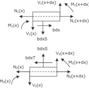
2.2.1.2. Governing equations. The local equilibrium of both adherends (see Figure 6) leads to the following system of six equations:

dNj bdx¼ ð#1Þ j T dVj bdx¼ ð#1Þ jþ1_S dMj dx þ Viþ ej 2 bT¼ 0 8 > > < > > : ; j¼ 1; 2 ð18Þ

where, S is the adhesive peeling stress, V1 (V2) is the shear force in the adherend 1 (2) and

M1(M2) is the bending moment in the adherend 1 (2).

This local equilibrium is the one derived and employed by Goland and Reissner [17] in their classical theory. Furthermore, considering a possible extensional and bending coupling stiffness in the adherends, the constitutive equations are expressed as:

Nj¼ Aj duj dx# Bj d2_w j dx2 Mj¼ #Bj duj dxþ Dj d2_w j dx2 hj¼ dwj dx 8 > < > : ; j_{¼ 1; 2 ð19Þ}

with Aj as the extensional stiffness, Bj as the coupling stiffness, and Dj as the bending

stiff-ness.

Figure 5. Comparison of the adhesive shear stress distribution along the overlap between the present

1D-bar model with the analysis provided by Tsai and Morton [16].

It is assumed that !j¼ Aj2# B_jD_j is not equal to zero. The adhesive is considered as lin-ear elastic and is simulated by an infinite number of shlin-ear and transverse normal springs. The adhesive shear stress and the adhesive peeling stress are then expressed by:

T ¼ Gu2#u1#12e1h1#12e2h2 e S ¼ Ew1#w2 e ( ð20Þ where, E is the Young’s modulus of the adhesive, w1(w2) is the deflection of the adherend 1

(2) and h1(h2) is the bending angle of the adherend 1 (2).

2.2.1.3. Stiffness matrix of the BBe element. System of differential equations in terms of adhe-sive stresses. The Equation (19) is written as:

duj dx ¼ DjNjþBjMj !j d2_w j dx2 ¼ AjMjþBjNj !j ( ; j¼ 1; 2 ð21Þ

By combining Equations (18), (20), and (21), the following linear differential equation sys-tem, in terms of adhesive stresses, is obtained:

d3_T dx3 ¼ k1dT_dxþ k2S d4_S dx4 ¼ #k4S# k3dT_dx ( ð22Þ where, k1¼Gb_{e !}D1₁ 1þ A1e21 4D1 6 7 þD2 !2 1þ A2e22 4D2 6 7 þ e1B1 !1 # e2B2 !2 6 7 h i k2¼Gb_e e_2!1A₁1#e_2!2A₂2þ !B11þ B2 !2 6 7 h i k3¼Eb_e e_2!1A₁1#e_2!2A₂2þ _!B1₁þ_!B2₂ 6 7 h i k4¼Eb_{e !}A1₁þ_!A2₂ h i 8 > > > > > > > > < > > > > > > > > : ð23Þ

The system of differential Equation (22) can be uncoupled by differentiation and linear combination as: d6_S dx6# k1d 4_S dx4þ k4d 2_S dx2þ Sðk2k3# k1k4Þ ¼ 0 d dxð d6_T dx6# k1d 4_T dx4þ k4d 2_T dx2þ Tðk2k3# k1k4ÞÞ ¼ 0 ( ð24Þ This system is solved and the adhesive shear and peeling stresses are, thus, written as (see Appendix A):

pt SðxÞ ¼ K1e sx_{sinðtxÞ þ K} 2esxcosðtxÞ þ K3e#sxsinðtxÞ þK4e#sxcosðtxÞ þ K5erxþ K6e#rx : ; TðxÞ ¼ K1e sx_{sinðtxÞ þ K} 2esxcosðtxÞ þ K3e#sxsinðtxÞ þK4e#sxcosðtxÞ þ K5erxþ K6e#rxþ K7 : ; 8 > > > < > > > : ð25Þ

There are then 13 integration constants. However, by introducing these previous expres-sions of adhesive stresses in Equation (22), the integration constants of the adhesive peeling stress appear linked to those of adhesive shear stress as:

K1¼sðs 2_#3t2_#k 1Þ k2 K1þ tðt2_#3s2_þk 1Þ k2 K2¼ a1K1þ a2K2 K2¼ tð3s2_#t2_#k 1Þ k2 K1þ sðs2_#3t2_#k 1Þ k2 K2¼ #a2K1þ a1K2 K3¼ sð3t2_#s2_þk 1Þ k2 K3þ tðt2_#3s2_þk 1Þ k2 K4¼ #a1K3þ a2K4 K4¼tð3s 2_#t2_#k 1Þ k2 K3þ sð3t2_#s2_þk 1Þ k2 K2¼ #a2K3# a1K4 K5¼rðr 2_#k 1Þ k2 K5¼ a3K5 K6¼rðk1#r 2_Þ k2 K6¼ #a3K6 8 > > > > > > > > > > < > > > > > > > > > > : ð26Þ

Finally, seven independent integration constants remains: K1–K7.

Nodal displacements and forces. The determination of the stiffness matrix of BBe element requires the determination of nodal displacements and forces (see Figure 7). Following the resolution scheme in [18], the idea is to express the displacements and the forces in the adh-erends, as a function of the stress adhesives and of their derivatives. The computation is fully detailed in Appendix B. It is shown that a total number of 12 integration constants are finally involved: K1–K7, J1–J3,and J5–J6. The displacements in the adherends are then expressed as:

u1ðxÞ ¼ ~b1Tþ b1dSdx# b!2_K 7#6B1J0=! 2A1 x ! < =2 þJ5_!x þ J6 u2ðxÞ ¼ ~b2Tþ b2dSdxþ b!2_K 7þ6B2J0=! 2A2 x ! < =2 þ J5þJ!1ðe1þ e2Þ < =_x ! þJ6þ_2!J2ðe1þ e2Þ # K7 e₂1b~5þ e2 2b~6 6 7 w1ðxÞ ¼ ~b3 k4dT_dxþ k2d 2_S dx2 < = þ b5Sþ J0 _!x < =3 þJ1 _!x < =2 þJ2_!x þ J3 w2ðxÞ ¼ ~b4 k4dT_dxþ k2d 2_S dx2 < = þ b6Sþ J0 !x < =3 þJ1 !x < =2 þJ2!x þ J3 h1ðxÞ ¼ ~b5Tþ b5dSdxþ 3J0 x2 !3þ 2J1_!x2þ J2 !# K7b~5 h2ðxÞ ¼ ~b6Tþ b6dSdxþ 3J0 x2 !3þ 2J1_!x2þ J2 !# K7b~6 8 > > > > > > > > > > > > > > > < > > > > > > > > > > > > > > > : ð27Þ

The nodal displacements are then the values in x = 0 and x = Δ of Equation (27). The con-stitutive Equation (19) allow for the computation of normal and shear forces and of bending moments in both adherends:

N1ðxÞ ¼ ~a1dTdxþ a1d 2_S dx2# bK7x# 2B1LJ12þ A1JL5 N2ðxÞ ¼ ~a2dT_dxþ a2d 2_S dx2þ bK7xþ J1 #2B_L22þ A2e1_Lþe22 < = þ A2J_L5 M1ðxÞ ¼ ~a3dT_dxþ a3d 2_S dx2þ x L 6J0 L2 !1 A1þ bLK7 B1 A1 6 7 þ 2D1_LJ12# B1J_L5 M2ðxÞ ¼ ~a4dT_dxþ a4d 2_S dx2þ x L 6J0 L2 !2 A2# bLK7 B2 A2 6 7 þ J1 2D_L22# B2e1_Lþe22 < = # B2J_L5 V1ðxÞ ¼ #~a3d 2_T dx2# a3d 3_S dx3#1_L 6J0 L2 !1 A1þ bLK7 B1 A1 6 7 #e1b 2T V2ðxÞ ¼ #~a4d 2_T dx2# a4d 3_S dx3#1_L 6J0 L2 !2 A2# bLK7 B2 A2 6 7 #e2b 2T 8 > > > > > > > > > > > < > > > > > > > > > > > : ð28Þ

The nodal forces are then the values in x = 0 and x = Δ of Equation (28).

Stiffness matrix. The coefficients of the stiffness matrix of the BBe element are obtained by differentiating each nodal force by each nodal displacement:

KBBe ¼ @Qr @us h i @Qr @ws h i @Qr @hs h i @Rr @us h i @Rr @ws h i @Rr @hs h i @Sr @us h i @Sr @ws h i @Sr @hs h i 0 B B B @ 1 C C C A ; r; s¼ i; j; k; l ð29Þ

where, Qσ(Rσ) is the nodal normal (shear) forces and Sσ are the nodal bending moments.

The 12 nodal displacements (uγ, γ = 1:12) and the 12 nodal forces (Qα, α = 1:12) are

expressed as functions of the 12 independent integration constants (Cβ, β = 1:12). The nodal

forces depend linearly on integration constants, as well as the nodal displacements. Thus, the integration constants depend linearly on the nodal displacements (Equation (30)), enabling the determination of 144 coefficients of KBB(Equation (31)):

Qa¼ X12 b¼1 nabCb and Cb¼ X12 c¼1 m0bcuc ð30Þ @Qa @ud ¼ X nab X m0bc @uc @ud ð31Þ But, @uc @ud¼ dcd¼ 1 if c¼ d 0 if c–d & )@Qa @ud ¼ P12 b¼1 nabm0bd m0 bd¼ Cbðud¼ 1 ; uc–d¼ 0Þ ¼ Cbð0; . . . ; 0; ud¼ 1; 0; . . . ; 0Þ ð32Þ

The coefficients of KBBare, thus, obtained through:

½KBB'_a;d¼ @Qa @ud ¼ X12 b¼1 nabCbð0; . . . ; 0; ud¼ 1; 0; . . . ; 0Þ ð33Þ

Practically, Cβ(0, … , 0,uδ= 1,0, … , 0) is automatically generated by looping on the 12

canonical vectors of displacement, through the following inversion: Cβ[(0, … , 0, uδ= 1, 0,

2.2.1.4. Considering the shear stress in the adherends. This section describes how to con-sider the shear effects in the adherends by simply adapting a finite number of previous param-eters. The approach is based on the assumption of a linear variation of shear stresses in the adherends, according to Tsai and Morton theory [16]. From Equation (11), the shear strain γ1

for the upper adherend and γ2for the lower one are expressed as:

cj¼ Tj Gj¼ # 1 2 1þ ð#1Þ j 2yj ej 3 _{4 T} Gj¼ @ujðx; yjÞ @yj þ dwj dx; j¼ 1; 2 ð34Þ

The integration of normal displacements with respect to dyjprovides:

u1ðx; y1Þ ¼ u1ðx; 0Þ #_2GT₁ y1# y2 1 e1 h i # y1dw_dx1 u2ðx; y2Þ ¼ u2ðx; 0Þ #_2GT₂ y2þ y2 2 e2 h i # y2dw_dx2 8 < : ð35Þ Taking into account the previous shape of normal displacements, the constitutive equa-tions of adherends (19) become:

N1¼ A1du_dx1# B1d 2_w 1 dx2 # C1dT_dx N2¼ A2dudx2# B2d 2_w 2 dx2 # C2dTdx M1¼ #B1du_dx1þ D1d 2_w 1 dx2 þ C10dTdx M2¼ #B2du_dx2þ D2d 2_w 2 dx2 þ C20dTdx C1¼e1_2eB1₁#D_G11 C2¼e2_2eB2₂þD_G22 C0 1¼ e1D1#F1 2e1G1 C₂0 ¼ #e2D2þF2 2e2G2 8 > > > > > > > > > > > > > > > > < > > > > > > > > > > > > > > > > : ð36Þ with, Fj¼ b 4 X nj pj¼1 Qpj j h4pj# h 4 pj#1 h i ; j¼ 1; 2 ð37Þ

where, hpi – the y-coordinates of the pthj layer and Qj pi

is the reduced rigidity matrix of the pthply of adherends j.

As detailed in Appendix C, the modification of the shape of the constitutive equations of adherends results in modification of suitable constants only.

2.2.2. Assembly and validation on the exemplified single-lap joint

The single-lap bonded joint is meshed as following: (i) the overlap is meshed with 1 BBe ele-ment, (ii) each adherend outside the overlap is meshed with 1 bar element. This mesh leads to a total number of six nodes (see Figure 8).

The stiffness matrix of the single-lap joint is then assembled, according to the classical FE rules, from the stiffness matrix of each element. The stiffness matrix of a beam element, named Kbeam, is written (according to [15]):

Kbeam¼ Aj lj # Aj lj 0 0 #Bj lj Bj lj #Aj lj Aj lj 0 0 Bj lj # Bj lj 0 0 12 l3 j ! Aj # 12 l3 j ! Aj 6 l2 j ! Aj 6 l2 j ! Aj 0 0 #12 l3 j ! Aj 12 l3 j ! Aj # 6 l2 j ! Aj # 6 l2 j ! Aj #Bj lj Bj lj 6 l2 j ! Aj # 6 l2 j ! Aj 1 lj 3! Ajþ D j 3 4 1 lj 3! Aj# D j 3 4 Bj lj # Bj lj 6 l2 j ! Aj # 6 l2 j ! Aj 1 lj 3! Aj# Dj 6 7 1 lj 3! Ajþ D j 3 4 0 B B B B B B B B B B B B B B B B B B B B B @ 1 C C C C C C C C C C C C C C C C C C C C C A ; j¼ 1; 2 ð38Þ

Following the classical FE rules, the boundary conditions are then applied to the single-lap bonded joint, which is simply supported at both extremities, fixed according to the x-axis at one extremity and free at the other one, where a force f = 10 N is applied (see Figure 8). A total number of DoF equal to 15 is then involved. The resolution consists then in inverting a 15+ 15 linear system.

The adhesive stress distribution predicted by [16] is compared to the present model pre-dictions for the single-lap bonded joint defined in Figure 1 and Table 1. In order to perform a comparison on exactly the same hypotheses, the length outside the overlap is computed according to the Goland and Reissner theory [17], resulting in a same bending moment at both overlap ends (for a beam approach) under the applied force (li= 91 mm). Moreover, the

Figure 8. Bonded assembly and boundary conditions.

Figure 9. Comparison of the adhesive shear stress distribution along the overlap between the 1D-beam

factor C_j0 is set to zero. The superimposition of curves shown in Figure 9 allows for the con-clusion that the same hypotheses lead to the same results.

3. Assuming an elasto-plastic adhesive material

3.1. Numerical approach

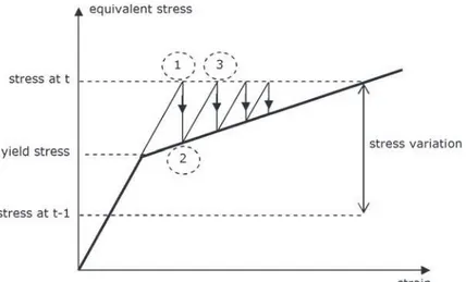
In this section, the adhesive, employed in the bonded area, is assumed to have an elasto-plas-tic behavior. To take into account this nonlinear behavior, an iterative procedure [19] is imple-mented, starting from the previous linear elastic formulation. This iterative procedure is illustrated in Figure 10, for a stress step resulting in a current elastic stress state characterized by an equivalent stress superior to the yield stress. This current elastic stress state is obtained through the linear computation F = KU, representing the first step of the procedure. The sec-ond step correspsec-onds to the projection of the equivalent stress to the elastic stress state on the yield function allowing for the computation for a first residue R, relevant to the difference between the elastic stress state and the projected stress state. In this paper, this second step is presented assuming an elastic perfectly plastic behavior. The third step consists in imposing to the structure the residue, such as R = KU. This procedure is repeated, while the norm of the residue is higher than a prescribed threshold. The residues have thus to be computed. Hereafter, the equivalent stress chosen for the 1D-bar model is the shear stress (maximal stress criterion), while for the 1D-beam model, the criterion is the von Mises equivalent stress.

3.2. Example of application for structures: single-lap joint, in-plane loading

3.2.1. Equilibrium of the structure

For both 1D-bar and 1D-beam models, the equilibrium of the structure is such that at any abscissa along the overlap, the sum of normal and shear forces in the adherends is constant:

N1þ N2¼ N2ðLÞ ¼ N1ð0Þ ¼ f

V1þ V2¼ V2ðLÞ ¼ V1ð0Þ ð39Þ

For both 1D-bar and 1D-beam models, the local equilibrium of adherends, according to the x-axis and y-axis allows for a relationship between the normal and shear forces in the adherends and the adhesive shear and peeling stresses:

N2ðxÞ # N2ð0Þ ¼ N2ðxÞ ¼ b Rx 0Tdx V2ðxÞ # V2ð0Þ ¼ V2ðxÞ ¼ b Rx 0Sdx ð40Þ In particular, the area under the shear stress distribution along the overlap (named S0)

multiplied by the overlap width is equal to the applied force:

S0¼ b

Z L 0

TðxÞdx ¼ f ð41Þ

This last equilibrium requirement is used in the iterative procedure to ensure its conver-gence.

3.2.2. Determination of the nodal residue

Case with a mesh with n-macro-elements. The bonded overlap is regularly meshed in n macro-elements, such nΔ = L (see Figure 11). A total number of 2n + 2 nodes are involved.

For 1D-bar case. The elastic shear stress on the kth _{node is computed through the nodal}

displacements and is quoted Te(k). The projected stress on the yield function is named Tp(k).

The difference between these two stresses is named δT(k):

8k 2 ½2; 2n þ 3'; dT_{ðkÞ ¼ T}eðkÞ # TpðkÞ ð42Þ

Along the elastic zones, this difference is equal to zero. Moreover, this difference is the same for both nodes located at the same abscissa:

8k 2 ½2; 2n þ 3'; 8p 2 ½1; n þ 1'; d^TðpÞ ¼ dTðk ¼ 2pÞ ¼ dTðk ¼ 2p þ 1Þ ð43Þ Before the application of the prescribed displacements, the relevant components of the residue vector to normal nodal forces are:

Rð0Þ ¼ 0 for p2 ½1; n þ 1'; Rð2pÞ ¼ #b! / d^TðpÞ Rð2p þ 1Þ ¼ b! / d^TðpÞ & Rð2n þ 4Þ ¼ f ð44Þ

For 1D-beam case. The elastic shear and peeling stresses on the kth node are computed through the nodal displacements and are named Te(k) and Se(k), respectively. The projected

shear and peeling stresses on the yield function are named Tp(k) and Sp(k), respectively. As

for the 1D-bar case, the difference between the elastic peeling stress and the projected peeling stress is:

8k 2 ½2; 2n þ 3'; 8p 2 ½1; n þ 1';

d^SðpÞ ¼ dSðk ¼ 2pÞ ¼ dSðk ¼ 2p þ 1Þ ¼ SeðkÞ # SpðkÞ ð45Þ

Before the application of the prescribed displacements, the relevant components of the residue vector to normal nodal forces are given in Equation (44), whereas those relevant to the shear nodal forces are:

Rð0Þ ¼ 0 for p2 ½1; n þ 1'; Rð2pÞ ¼ #b! / d^SðpÞ R_{ð2p þ 1Þ ¼ b! / d^SðpÞ} & Rð2n þ 4Þ ¼ 0 ð46Þ

3.2.2.1. Case with a mesh with one macro-element. The bonded overlap is meshed with one macro-element only, which implies a total number of six nodes (see Figure 5).

For the 1D-bar case. The elastic shear stress is computed at any abscissa x with Equation (6) and is named Te(x). The projected stress on the yield function is named Tp(x). The

differ-ence between these two stresses is named δT(x). The residue is obtained after summation of δT(x) for any abscissa such δT(x) ≠ 0. More precisely, if the elastic zone is included between x1 and x2 (see Figure 12), before the application of the prescribed displacements, the

components of the residue vector are:

Rð0Þ ¼ 0 Rð2Þ ¼ #bRx1 0 dTðxÞdx Rð3Þ ¼ bRx1 0 dTðxÞdx R_{ð4Þ ¼ #b}RL x2dTðxÞdx Rð5Þ ¼ bRL x2dTðxÞdx 8 > > > < > > > : R_{ð6Þ ¼ f} ð47Þ

For the 1D-beam case. The elastic shear stress and peeling stresses are computed at any abscissa x with Equation (25) and are named Te(x) and Se(x), respectively. The projected shear

and peeling stresses on the yield function are named Tp(x) and Sp(x). The difference between

the elastic and projected shear and peeling stresses are named δT(x) and δS(x). The relevant components of residue vector to normal nodal forces are the same as those given in Equation (47). In the same way, before the application of the prescribed displacements, the relevant components of residue vector to shear nodal forces are:

Rð0Þ ¼ 0 Rð2Þ ¼ #bRx1 0 dSðxÞdx Rð3Þ ¼ bRx1 0 dSðxÞdx Rð4Þ ¼ #bRL x2dSðxÞdx R_{ð5Þ ¼ b}RL x2dSðxÞdx 8 > > > < > > > : Rð6Þ ¼ 0 ð48Þ 3.2.3. Projected stresses

In the 1D-bar model, only one adhesive stress component is involved. The projected stress depends only on the yield function following the maximal stress criterion. In the 1D-beam model, the peeling stress and the shear stress are considered allowing the computation of the von Mises equivalent stress, named σe, which is chosen as yield criterion:

re¼ ffiffiffiffiffiffiffiffiffiffiffiffiffiffiffiffiffiffi 3T2 e þ Se2 p ð49Þ The equivalent projected stress, named σp, is computed as a function of Tpand Spas:

rp¼ ffiffiffiffiffiffiffiffiffiffiffiffiffiffiffiffiffiffi 3T2 pþ S2p q ð50Þ When the yield criterion is exceeded, the equivalent stress is expressed as:

3T2 e þ S 2 e ¼ r 2 pþ Q 2 ð51Þ where, Q characterizes the exceeding of yield criterion.

The Equation (51) can be rearranged as: r2 p¼ 3T 2 e þ S 2 e # 3T2 e þ S 2 e 3T2 e þ S2e Q2 ð52Þ leading to:

r2 p¼ 3 T 2 e # T2 e 3T2 e þ Se2 Q2 3 4 þ S2 e# S2 e 3T2 e þ S2e Q2 3 42 ð53Þ Finally, the projected stresses are written as functions of the elastic stresses and yield cri-terion excess: Tp¼ signðTeÞ Te ffiffiffiffiffiffiffiffiffiffiffiffiffiffiffiffiffiffiffi 1# Q2 3T2 eþSe2 q Sp¼ signðSeÞ Se ffiffiffiffiffiffiffiffiffiffiffiffiffiffiffiffiffiffiffi 1# Q2 3T2 eþSe2 q 8 < : ð54Þ 3.2.4. Solution procedure

The solution procedure is summarized hereafter. A. Linear elastic computation

A.1 The stiffness matrix of the structure is computed (see Section 2). A.2 Initialization of variables:

• _{fR= f}

• _{R = F, such}t_{F = (0 … 0 f ).}

A.3 Computation of U = K#1R, after applying the boundary conditions in displacement. A.4 Computation of adhesive elastic stresses for any abscissa of overlap (see Section 2). A.5 Computation of adhesive equivalent stress σe.

A.6 Computation of S0(see Section 3.2.1).

B. Yielding test

if σeis inferior to the adhesive yield stress then end,

else computation of Q as the difference of the adhesive equivalent stress and the adhesive yield stress.

C. Plastic loop

C.1 Projection of adhesive stresses on the yield function (see Section 3.2.3).

C.2 Computation of the difference between the adhesive elastic stresses and the adhesive pro-jected stress (see Section 3.2.2).

C.3 Update of R (see Section 3.2.2).

C.4 If norm(R) < threshold_2 then go to D, else go to A.3. D. Global equilibrium

if abs(S0# f) > threshold_2 then fR= fR# (S0# f ) and go to A.3,

else end.

4. Comparison with FE predictions

4.1. Overview

In order to assess and to validate both models based on a simplified approach, FE models are developed using SAMCEF FE code v14–1. For validation purposes, a 1D-bar FE model is compared to the current 1D-bar model, without considering any shear deformations in the adherends. For assessment, a PS and a 3D FE model are compared with the current 1D-beam model, including a linear variation of the shear stress in the adherends. The joint is clamped at one end and free to move at the other end in the longitudinal direction only, where the load

is applied. A force per unit of width unit of 10 N.mm#1 is applied. The geometry of the sin-gle-lap joint is that which is introduced in Figure 1 and Table 1. For the 3D FE model, the width of structure is taken equal to 1 mm. The adherends are assumed to be linear elastic and the material characteristics are given in Table 1. The adhesive is considered as elastic per-fectly plastic. The adhesive elastic parameters are given in Table 1. In the 1D-bar analysis, the adhesive remains in its elastic domain if the shear stress is inferior to 0.55 MPa. For all the other analyses, the von Mises yield criterion is employed with a yield stress of 1.6 MPa. The FE computations are geometrically linear. 100 macro-elements are employed in the mod-els based on the simplified approaches. It is indicated (not discussed here) that a mesh with 1 macro-element leads to almost the same results for all the cases tested. For the PS and 3D FE models, the stresses are measured along the middle line of the adhesive layer and in the sym-metry plane for the 3D FE model. Indeed, in contrast to refined PS or 3D FE models [20], the models based on the simplified approach are not able to capture the edge effects at the interfaces with the adherends or at the free edges.

4.2. Description of FE models

4.2.1. 1D-bar FE model

The adherends are simulated by beam elements (SAMCEF type T022). The adhesive layer is simulated by bush elements, which connect the beam elements involved along the overlap. To simulate the 1D-bar model, the displacements according to the y-axis and the z-axis are fixed. In order for the bush elements to work in shear only, all the stiffnesses are set to unity except that for the shear mode. The latter is computed according to [21]. A preliminary study (not presented in this paper) showed that a number of 100 bush elements regularly distributed along the overlap allow for accurate results at restricted computational time cost. In the adher-ends, 204 beam elements are set. Moreover, the unbalanced configuration such that e2= 2e1= 4.8 mm is under consideration.

4.2.2. PS FE model

The adherends and the adhesive are simulated by quadrangular elements (SAMCEF type T015) under PS conditions. The elements chosen have linear interpolation functions and four internal modes. The normal integration scheme is chosen. As the adhesive stresses signifi-cantly vary at the overlap edges, the mesh is thus refined in this area though a progressive mesh. The smallest element in the adhesive layer is then located at both overlap ends and has an aspect ratio equal to 1. A nominal number of four elements in the adhesive layer is chosen (see Section 4.2.3) leading to a minimal size of 0.1 mm+ 0.1 mm. Furthermore, a transition ratio equal to one is set at the interface with the adhesive and a progressive mesh is adopted in the adherends.

4.2.3. 3D FE model

The adherends and the adhesive are simulated by 3D brick elements (SAMCEF type T008). The elements chosen have linear interpolation functions and nine internal modes (8 nodes and 24 DoF). The normal integration scheme is chosen. The mesh of the 3D model consists in an extrusion in the width direction of the PS FE model mesh. Symmetry conditions are applied in an external plane, the normal of which is the direction of extrusion. The stresses are mea-sured along the middle line of the adhesive layer and on the symmetry plane.

The maximum value of adhesive shear and peeling stresses depends on the mesh density. As the objective of this comparison of PS and 3D FE predictions is to assess the relevance of the 1D-beam model, the dependency of shear and peeling peaks on the mesh density has to be addressed. The study consists then in measuring the maximum values of the adhesive shear and peeling stresses as a function of the number of elements in the adhesive layer thick-ness. The number of elements in the adhesive layer varies, while keeping the aspect ratio of the smallest element in the adhesive layer (located at both overlap ends) equal to 1. It is shown that the shear (peeling) peak increases (decreases) with the increasing number of ele-ments in the adhesive layer (see Figure 13). However, this increasing or decreasing tendency significantly slows down with the increasing number of elements. Table 2 shows changes to

Figure 13. Shear (a) and peeling (b) peaks on the adhesive middle line as a function of the number of

Table 2. Relative difference to the case with 32 elements, when the number of elements in the adhesive thickness varies.

Number of elements

Relative difference to the case with 32 elements

Shear stress peak (%) Peeling stress peak (%)

2 #3.94 25.8

4 _#1.16 2.80

8 _{#0.559 #1.83}

16 _#0.361 0.372

Figure 14. Shear (a) and peeling (b) peaks on the adhesive upper (or lower) line compared to the

shear (a) and peeling (b) peak on the adhesive center line, as a function of the number of elements in the adhesive thickness.

the adhesive shear and peeling peaks for varying number of elements, relative to those for 32 elements. It can be observed that these relative differences are quite low, except for the peel-ing peak for the case with two elements. It could be thought that the hypothesis of an elastic perfectly plastic adhesive material behavior allows for the saturation of the adhesive peak stresses, contributing to low variations. In order to understand the elevated difference on the peak stress for the case with two elements, the shear and peeling peak adhesive stress on the upper (or lower) external line of the adhesive layer is measured while the number of elements varies. These peaks on the adhesive upper (or lower) line are located at overlap ends, as for the adhesive middle line. As shown in Figure 14, whereas the increase of the number of ele-ments in the adhesive layer decreases the relative difference to the middle line on the shear peak, this relative difference increases significantly. The influence of the edge effect on the adhesive stress at the middle line thus seems to be reduced by refining the mesh in the adhe-sive thickness. Finally, it is considered that almost steady values for shear and adheadhe-sive peaks can be obtained, when the side height of the smallest element in the adhesive layer is inferior to 0.1 mm (i.e. four elements in an adhesive thickness of 0.4 mm).

4.3. Comparison of results

4.3.1. 1D-bar present model vs. 1D-bar FE model

Firstly, it is indicated (not presented here) that, when the adhesive is supposed linear elastic, the 1D-bar present model (without any shear in the adherends) and 1D-bar FE model provide exactly the same adhesive shear stress distribution along the overlap. Considering the elasto-plastic behavior of the adhesive, the 1D-bar present model (without any shear in the adher-ends) and 1D-bar FE model provide exactly the same adhesive shear stress distribution along the overlap, for the balanced and unbalanced configuration, as shown in Figures 15 and 16, respectively.

4.3.2. 1D-beam present model vs. PS and 3D FE models

The 1D-beam present model with a linear shear stress in the adherends is compared to the PS and 3D FE models, in case of a balanced configuration for example. The distribution of the

Figure 15. Comparison of the adhesive shear stress distribution along the overlap between the 1D-bar

adhesive shear, peeling and von Mises stresses along the overlap are provided in Figures 17– 19. Although the stress tensor component number is restricted to two in the 1D-beam present model, a good agreement is shown.

4.3.3. Evolution of adhesive stress distribution with the applied load

In order to illustrate the effect of plasticity of the adhesive stress distribution, the adhesive shear, peeling, and von Mises stress distribution obtained with the 1D-beam present model are provided in Figures 20–22, respectively, at two intermediate applied loads (5 and 7 N. mm#1). The structure chosen is the unbalanced configuration such that e2= 2e1= 4.8 mm.

The adhesive layer is meshed with four elements in its thickness (leading to a side length of 0.1 mm for the smallest element). Furthermore, the stress distributions at an applied load of

Figure 16. Comparison of the adhesive shear stress distribution along the overlap between the 1D-bar

present model and 1D-bar FE models, on an unbalanced structure.

Figure 17. Comparison of the adhesive shear stress distribution along the overlap between the

10 N.mm#1 are compared to those predicted by the 3D FE models, resulting in a good agree-ment. Moreover, it appears that the adhesive stress peak saturation is balanced by the increase of the minimal adhesive stress level reached along the overlap.

4.4. Assessment of the relevance of the model

In order to assess the relevance of the present 1D-beam model, unbalanced configurations such that e2= 2e1= 4.8 mm with isotropic adherends are under consideration. The study

described in this section consists of measuring the relative differences between the 3D FE model predictions and the 1D-beam model predictions, in terms of adhesive shear and peeling stresses, when: (i) the adherend stiffness varies then (ii) the adhesive thickness varies.

Con-Figure 18. Comparison of the adhesive peeling stress distribution along the overlap between the

1D-beam present model and PS and 3D FE models, on a balanced structure.

Figure 19. Comparison of the adhesive Von Mises stress distribution along the overlap between the

cerning the influence of the adherend stiffness, the variation of the adherend stiffness is achieved by fixing the Young’s modulus of the adherend 1 at its value in Table 1 (E1= 72 GPa), while the Young’s modulus of the adherend 2 is varying such E2= (0.5, 1,

2, 3)+ E1. In the 3D FE model, the adhesive layer is meshed with four elements in its

thick-ness (leading to a side length of 0.1 mm for the smallest element). As shown in Table 3, the 1D-beam model provides adhesive shear and peeling peaks very close to those predicted by the 3D FE model, with relative differences inferior to 10%. Moreover, in terms of stress dis-tribution along the overlap, a good correlation is obtained, as shown in Figures 23–25 for the case E2/E1= 3. In particular, the overstress for abscissas close to zero, due to the unbalance of

Figure 20. Comparison of the adhesive shear stress distribution along the overlap between the

1D-beam present model and PS and 3D FE models, on an unbalanced structure. The distributions at various intermediated applied forces are shown.

Figure 21. Comparison of the adhesive peeling stress distribution along the overlap between the

1D-beam present model and PS and 3D FE models, on an unbalanced structure. The distributions at various intermediated applied forces are shown.

Table 3. Relative difference to the FE predictions, when the adherend stiffness varies.

E1/E2

Relative difference to the 3D FE model predictions

Shear stress peak (%) Peeling stress peak (%)

0.5 0.642 #4.93

1 #2.57 #1.46

2 #3.53 7.41

3 #1.83 5.00

Figure 22. Comparison of the adhesive von Mises stress distribution along the overlap between the

1D-beam present model and PS and 3D FE models, on an unbalanced structure. The distributions at various intermediated applied forces are shown.

Figure 23. Comparison of the adhesive shear stress distribution along the overlap between the

Figure 24. Comparison of the adhesive peeling stress distribution along the overlap between the 1D-beam present model and 3D FE models, on an unbalanced structure.

Figure 25. Comparison of the adhesive von Mises stress distribution along the overlap between the

1D-beam present model and 3D FE models, on an unbalanced structure.

Table 4. Relative difference to the FE predictions, when the adhesive stiffness varies.

Adhesive thickness (mm)

Relative difference to the 3D FE model predictions

Shear stress peak (%) Peeling stress peak (%)

0.1 0.336 #18.7

0.2 1.25 #8.25

0.3 0.224 1.56

0.4 #2.25 3.16

the joint, is correctly retrieved. Concerning the influence of the adhesive thickness, five adhe-sive layer thicknesses are chosen: 0.1, 0.2, 0.3, 0.4, and 0.5 mm. In the 3D FE model, the number of elements in the adhesive thickness is taken such that the side length of the smallest element is equal to 0.5 mm (e.g. eight elements in an adhesive thickness of 0.4 mm). As shown in Table 4, the 1D-beam model provides adhesive shear and peeling peaks very close to the ones predicted by the 3D FE model (see Figures 20–22, for the case e = 0.4 mm), with relative differences inferior to 10%, except for the peeling peak for an adhesive thickness of 0.1 mm. However, when the adhesive thickness is equal to 0.1 mm, it is meshed with only two elements, resulting in a significant influence of edge effects on the peeling stress at over-lap ends when measured in the adhesive middle line (see Section 4.2.3).

Finally, the computation times required for the FE models of Section 4.2.3, when the number of elements in the adhesive thickness varies, are expressed as functions of the compu-tation time recorded for the 1D-beam model (equal to 1.3 s). All the compucompu-tations are per-formed on the same computer (HP Z800). Table 5 shows that the less refined mesh is consuming 49 times more of computation time than the 1D-beam model. Nevertheless, it is underlined that the 3D FE models allow for a more refined stress analysis than the simplified approaches.

5. Conclusion

A 1D-bar and 1D-beam simplified approach for the stress analysis of bonded joints involv-ing an elasto-plastic adhesive is presented and illustrated for the sinvolv-ingle-lap joint configura-tion. The example of the single-lap bonded joint configuration should not be seen as a restriction, since various single-lap geometries could be simulated through simple manipula-tions of the structure stiffness matrix. The simplified approach, relying on the simplifying hypotheses provided in Section 2.1.1.1 and Section 2.2.1.1, is based on the formulation of a four-node macro-element able to simulate a full bonded overlap. Firstly, bar and 1D-beam macro-elements are formulated assuming a linear elastic adhesive behavior and taking into account a linear variation of the shear stress in the adherends. It is shown that the same hypotheses lead to the same results when the adhesive stress distributions along the overlap are compared with the reference ones. Secondly, an iterative procedure, employing the linear elastic computation of the stiffness matrix, is presented to take into account an elasto-plastic adhesive behavior. Assuming a yield function (elastic perfectly plastic behavior) and a yield criterion, the residue vector is computed through the projection of the current stress state, up to reaching equilibrium for a prescribed tolerance. Finally, the results provided by the models based on the simplified approach are compared to those of 1D-bar, PS, and 3D FE models, assuming an elastic perfectly plastic adhesive behavior. A good agreement is shown.

Table 5. Comparisons of computation times between the 3D FE models and the 1D-beam model

(1.3 s).

3D FE models

Number of elements in the adhesive thickness

2 4 8 16 32

Computation time in s 6.40E+01 4.30E+02 3.90E+03 7.42E+04 3.08E+05

Number of times higher than for 1D-beam model

Nomenclature and units

Aj extensional stiffness (N) of the adherend j

Bj extensional and bending coupling stiffness (N mm) of the adherend j

Dj bending stiffness (N mm

2

) of the adherend j

Ej Young’s modulus (MPa) of the adherend j

E Young’s modulus (MPa) of in the adhesive

F vector of forces

G Coulomb’s modulus (MPa) of the adhesive

Gj Coulomb’s modulus (MPa) of the adherend j

K stiffness matrix

KBBa stiffness matrix of the bonded-bars element

KBBe stiffness matrix of the bonded-beams element

L length (mm) of the overlap

Mj moment (N mm) in the adherend j around the z direction

Nj force (N) in the adherend j in the x direction

Qσ nodal normal force (N) applied to the node σ in the x direction (σ = i, j, k, l)

Rσ nodal shear force (N) applied to the node σ in the y direction (σ = i, j, k, l)

Sσ nodal bending moment (N mm) applied to the node σ around the z direction (σ = i, j, k, l)

S adhesive peel stress (MPa)

T adhesive shear stress (MPa)

U vector of displacements

Vj shear force (N) in the adherend j in the y direction

b width (mm) of the adherends

e thickness (mm) of the adhesive

ej thickness (mm) of the adherend j

f force (N) applied to the joint in the x direction

lj length (mm) of the beam outside the overlap of the adherend j

n number of macro-elements

uj displacement (mm) of the adherend j in the x direction

ua displacement (mm) of the node a in the x direction (a = i, j, k, l)

wj displacement (mm) of the adherend j in the y direction

wa displacement (mm) of the node a in the y direction (a = i, j, k, l)

Δ length (mm) of a macro-element

hj angular displacement (rad) of the adherend j around the z direction

ha angular displacement (rad) of the node a around the z direction (a = i, j, k, l)

(x, y, z) direct orthonormal base

Acknowledgement

The three first authors gratefully acknowledge the SOGETI HIGH TECH engineers and managers for their support involved in the development of JoSAT (Joint Stress Analysis Tool) internal research program.

References

[1] van Ingen JW, Vlot A. Stress analysis of adhesively bonded single lap joints. Delft University of Technology; 1993. (Report LR-740).

[2] Tsai MY, Morton J. An evaluation of analytical and numerical solutions to the single-lap joint. Int. J. Solids Struct. 1994;31:2537–2563.

[3] da Silva LFM, das Neves PJC, Adams RD, Spelt JK. Analytical models of adhesively bonded joints-part I: literature survey. Int. J. Adhes. Adhes. 2009;29:319–330.

[4] Hart-Smith LJ. Adhesive-bonded single-lap joints. Hampton (VA): National Aeronautics and Space Administration, Langley Research Center; 1973. (NASA CR 112236).

[5] Bigwood DA, Crocombe AD. Non-linear adhesive bonded joint design analysis. Int. J. Adhes. Adhes. 1990;10:31–41.

[6] Adams RD, Mallick V. A method for the stress analysis of lap joints. J. Adhes. 1992;38:199–217. [7] Tong L, Kuruppu M, Kelly D. Analysis of adhesively bonded composite double lap joints. J.

Ther-moplast. Compos. 1997;10:61–75.

[8] Mortensen F. Development of tools for engineering analysis and design of high-performance FRP-composite structural elements [PhD thesis]. Aalborg: Aalborg University; 1998.

[9] Smeltzer SS III. An inelastic methodology for bonded joints with shear deformable, anisotropic adherends [PhD thesis]. Raleigh (NC): North Carolina State University; 2003.

[10] Oterkus E, Barut A, Madenci E, Smeltzer SS III, Ambur DR. Nonlinear analysis of bonded com-posite single-lap joints. Paper presented at: 45th AIAA/ASME/ASCE/AHS/ASC Structures, Struc-tural Dynamics & Materials Conference; 2004 Apr 19–22; Palm Springs, CA.

[11] Yang C, Huang H, Tomblin JS, Sun W. Elastic-plastic model of adhesive-bonded single-lap com-posite joints. J. Compos. Mater. 2004;38:293–309.

[12] Paroissien E, Sartor M, Huet J. Hybrid (bolted/bonded) joints applied to aeronautic parts: analytical one-dimensional models of a single-lap joint. In: Tichkiewitch S, Tollenaere M, Ray P, editors. Advanced in integrated design and manufacturing in mechanical engineering II. Dordrecht: Springer; 2007. p. 95–110.

[13] Paroissien E, Sartor M, Huet J, Lachaud F. Analytical two-dimensional model of a hybrid (bolted/ bonded) single-lap joint. J. Aircraft. 2007;44:573–582.

[14] Stapleton SE. The analysis of adhesively bonded advanced composite joints using joint finite ele-ments [PhD thesis]. Ann Arbor (MI): University of Michigan; 2012.

[15] Paroissien E, Da Veiga A, Laborde A. An 1D-beam approach for both stress analysis and fatigue life prediction of bonded joints. In: Komorowski J, editor. ICAF 2011 structural integrity: influence of efficiency and green imperatives. Proceedings of the 26th Symposium of the International Com-mittee on Aeronautical Fatigue; 2011 Jun 1–3; Montreal (Canada): Springer.

[16] Tsai MY, Morton J. Improved theoretical solutions for adhesive lap joints. Int. J. Solids Struct. 1998;35:1163–1185.

[17] Goland M, Reissner E. The stresses in cemented joints. J. App. Mech.-T ASME. 1944;11: A17–A27.

[18] Högberg JL. Mechanical behavior of single-layer adhesive joints – an integrated approach [Msc thesis]. Göteborg: Chalmers University of Technology; 2004.

[19] Lubliner J. Platicity theory. New York (NY): Macmillan; 1990.

[20] Cognard JY, Créac’hcadec R, Sohier L, Leguillon D. Influence of adhesive thickness on the behav-ior of bonded assemblies under shear loadings using a modified TAST fixture. Int. J. Adhes. Adhes. 2010;30:257–266.

[21] Dechwayukul C, Rubin CA, Hahn GT. Analysis of the effects of thin sealant layers in aircraft structural joints. AIAA J. 2003;41:2216–2228.

Appendix A

This appendix details the resolution of the differential equation system in Equation (24). The characteris-tic polynomial expression is:

P_{ðRÞ ¼ ^aR}3_{þ ^bR}2_{þ ^cR þ ^d ¼ 0} R¼ r2 ^ a¼ 1 ^ b¼ #k1 ^ c¼ k4 ^ d¼ k2k3# k1k4 8 > > > > > > < > > > > > > : ðA:1Þ

R03þ ^pR0_{þ ^q ¼ 0} ^ p¼ #k21 3þ k4 ^ q¼ #k1 27ð2k 2 1# 9k4Þ þ k2k3# k1k4 8 < : ðA:2Þ where, R0¼ R #k1 3 ðA:3Þ

and the determinant is:

^ !_{¼ ^q}2 þ 4 27^p 3 ðA:4Þ By defining: ^ u¼3 ffiffiffiffiffiffiffiffiffiffiffiffiffi #^qþpffiffiffi_!^ 2 q ^ v¼3 ffiffiffiffiffiffiffiffiffiffiffiffiffi #^q#pffiffiffi_!^ 2 q 8 < : ðA:5Þ

The roots of the reduced equation are written as: R0 1¼ ^u þ ^v R0 2¼ j^u þ"j^v R0 3¼ j 2_{^uþ j}2_^v 8 < : ðA:6Þ Consequently, the roots of the characteristic Equation (A.1) are given by:

R1¼ ^u þ ^v þk₃1¼ r2 R2¼ #1₂ð^u þ ^vÞ þk₃1þ i ffiffi 3 p 2ð^u # ^vÞ ¼ ðs þ itÞ 2 R3¼ #12ð^u þ ^vÞ þ k1 3# i ffiffi 3 p 2ð^u # ^vÞ ¼ ðs # itÞ 2 8 > < > : ðA:7Þ

Finally, the adhesive stresses have to be determined as:

SðxÞ ¼ K1esxsinðtxÞ þ K2esxcosðtxÞ þ K3e#sxsinðtxÞ

þK4e#sxcosðtxÞ þ K5erxþ K6e#rx

: ;

TðxÞ ¼ K1esxsinðtxÞ þ K2esxcosðtxÞ þ K3e#sxsinðtxÞ

þK4e#sxcosðtxÞ þ K5erxþ K6e#rxþ K7 : ; r¼ ffiffiffiffiffiffiffiffiffiffiffiffiffiffiffiffiffiffiffi^uþ ^v þk1 3 q s¼ ffiffiffiffiffiffiffiffiffiffiffiffiffiffiffiffiffiffiffiffiffiffiffiffiffiffiffiffiffiffiffiffiffi1 2ðReðR2Þ þ jR2jÞ q t_¼ ffiffiffiffiffiffiffiffiffiffiffiffiffiffiffiffiffiffiffiffiffiffiffiffiffiffiffiffiffiffiffiffiffi1 2ðjR2j # ReðR2ÞÞ q 8 > > > > > > > > > > > > < > > > > > > > > > > > > : ðA:8Þ Appendix B

With the Equations (18) and (19), it is possible to express the derivatives of the longitudinal and trans-verse displacements as functions of adhesive stresses and their derivatives:

d4_w 1 dx4 ¼ A10dT_dxþ B10S d4_w 2 dx4 ¼ A20dT_dxþ B20S d3_u 1 dx3 ¼ C10dT_dxþ D10S d3_u 2 dx3 ¼ C20dT_dxþ D20S 8 > > > < > > > : ðB:1Þ where, A10¼ #_2!b₁½2B1þ e1A1'; B10¼ #A!11b A20¼_2!b₂½2B2# e2A2'; B20¼A_!2₂b C10¼ #_2!b₁½e1B1þ 2D1'; D10¼ #B_!1₁b C20¼_2!b₂½#e2B2þ 2D2'; D20¼B_!2₂b 8 > > > < > > > : ðB:2Þ

To obtain the expressions of displacements in the adherends, Equation (B.1) has to be integrated. Before integrating Equation (B.1), the differential Equation (22) is written as:

S¼ 1 k2k3#k1k4 k3 d3_T dx3þ k1d 4_S dx4 D E dT dx¼ 1 k1k4#k2k3 k4 d3_T dx3þ k2d 4_S dx4 D E ( ðB:3Þ and introduced in Equation (B.1). The displacements in the adherends are then expressed as:

w1¼ A_ðk10k4#B10k3 1k4#k2k3Þ2 k4 dT dxþ k2 d2_S dx2 < = þA10k2#B10k1 k1k4#k2k3 Sþ J0 x ! < =3 þJ1 _!x < =2 þJ2_!xþ J3 h i w2¼ A_ðk20k4#B20k3 1k4#k2k3Þ2 k4 dT dxþ k2 d2_S dx2 < = þA20k2#B20k1 k1k4#k2k3 Sþ J0 x ! < =3 þJ1 _!x < =2 þJ2_!xþ J3 h i u1¼ C10_k1k_k4₄#D_#k210_k3k3TþC10_k1k_k42#D_#k210_k3k1dS_dxþ J4 _!x < =2 þJ5_!xþ J6 h i u2¼ C20_k1k_k4₄#D_#k220_k3k3TþC20_k1k_k42#D_#k220_k3k1dS_dxþ J4 _!x < =2 þJ5_!xþ J6 h i h1¼ A10_k1k_k4_4#k#B₂10_k3k3ðT # K7Þ þA_k10_1kk2₄#B_#k210_k3k1dS_dxþ 3J0x 2 !3þ 2J1_!x2þ J2 ! h i h2¼ A20_k1k_k4_4#k#B₂20_k3k3ðT # K7Þ þA_k20_1kk2₄#B_#k220_k3k1dS_dxþ 3J0x 2 !3þ 2J1_!x2þ J2 ! h i 8 > > > > > > > > > > > > > > < > > > > > > > > > > > > > > : ðB:4Þ

Fourteen new integration constants are involved. However, following the resolution scheme in [18], the total number of integration constants can be reduced to 12.

Firstly, the second equation of system (18) gives:

dN2 bdx¼ T ) A2 d2_u 2 dx2 # B2 d3_w 2 dx3 ¼ bT ðB:5Þ Hence: A2 2J4 !2# B2 6J0 !3 ¼ bK7) J4¼ b!2_K 7 2A2 þ 3B2J0 A2! ðB:6Þ

In the same way, by considering the adherend 2, it becomes: J4¼ # b!2_K 7 2A1 þ 3B1J0 A1! ðB:7Þ

Secondly, the difference between the transverse displacements of both adherends provides:

w1# w2¼ e ESþ ðJ0# J0Þ x ! 6 73 þðJ1# J1Þ x ! 6 72 þðJ2# J2Þ x !þ J3# J3 ðB:8Þ

According to the definition of the peeling stress, it becomes:

Ji¼ Ji; i¼ 1; 3 ðB:9Þ

The difference of the longitudinal displacements provide:

u2# u1# 1 2e1h1# 1 2e2h2¼ e GTþ PðxÞ ðB:10Þ

where, P(x) is a quadratic polynomial, all coefficients of which have to be equal to zero: J4# J4# 3 2e1 J0 !# 3 2e2 J0 !¼ 0 ðB:11Þ J5# J5# e1 J1 !# e2 J1 !¼ 0 ðB:12Þ J6# J6# e1 2 J2 !# e2 2 J2 !þ K7 k1k4# k2k3 k4 e₂1A10þe₂2A20 < = #k3 e₂1B10þe₂2B20 < = : ; ¼ 0 ðB:13Þ

The displacements in the adherends are then expressed under the shape of Equation (27), with: ~ b_1¼C10k4#D10k3 k1k4#k2k3 ; b1¼ C10k2#D10k1 k1k4#k2k3 ~ b_2¼C20k4#D20k3 k1k4#k2k3 ; b2¼ C20k2#D20k1 k1k4#k2k3 ~ b5¼ A10k4#B10k3 k1k4#k2k3 ; b5¼ A10k2#B10k1 k1k4#k2k3 ~ b6¼ A20k4#B20k3 k1k4#k2k3 ; b6¼ A20k2#B20k1 k1k4#k2k3 ~ b_3¼ b~5 k1k4#k2k3; ~ b_4¼ b~6 k1k4#k2k3 J0¼ b!3 1 A1þA21 6 7 3ðe1þe2Þþ6 B1_A1#B2_A2 6 7K7 8 > > > > > > > > > > > > > > > > < > > > > > > > > > > > > > > > > : ðB:14Þ

The constitutive Equation (19) allow for the computation of normal and shear forces and of bending moments in both adherends, under the shape of Equation (28) with:

~ a1¼ A1b~1# B1b~5; a1¼ A1b1# B1b5 ~ a2¼ A2b~2# B2b~6; a2¼ A2b2# B2b6 ~ a3¼ #B1b~1þ D1b~5; a3¼ #B1b1þ D1b5 ~ a4¼ #B2b~2þ D2b~6; a4¼ #B2b2þ D2b6 8 > > > < > > > : ðB:15Þ Appendix C

Modification in the BBe element, induced by a linear shear stress in the adherends. The Equation (21) is modified as:

du1 dx ¼ D1N1þB1M1þ½D1C1#B1C01' dT dx !1 d2_w 1 dx2 ¼ A1M1þB1N1þ½B1C1#A1C01'dTdx !1 du2 dx ¼ D2N2þB2M2þ½D2C2#B2C0₂'dTdx !2 d2_w 2 dx2 ¼ A2M2þB2N2þ½B2C2#A2C02'dTdx !2 8 > > > > > > < > > > > > > : ðC:1Þ

The expression of the adhesive shear stress then becomes: T _¼G~ e u2# u1# 1 2e1h1# 1 2e2h2 < = ~ G¼ G 1þn2 n2¼3 8 G e e1 G1þ e2 G2 h i 8 > > < > > : ðC:2Þ

Moreover, the system of differential equations in terms of adhesive stresses (Equation (22)) becomes: d3_T dx3 ¼ k10dTdxþ k20S d4_S dx4¼ #k40S# k03 dT dx ( ðC:3Þ with, k0 1¼ k1 1#aT k0 2¼ k2 1#aT k0 3¼ k3þ k10k5 k0 4¼ k4þ k20k5 k5¼E_e B2C2#A2C20 !2 # B1C1#A1C10 !1 h i aT ¼ ~ G e D1C1#B1C01 !1 # D2C2#B2C20 !2 þ e1 2 B1C1#A1C10 !1 þ e2 2 B2C2#A2C02 !2 h i 8 > > > > > > > > > > < > > > > > > > > > > : ðC:4Þ

Then, the expressions of constants of Equation (B.2) are modified together with the expressions of displacements in Equation (27) accordingly:

A10¼ #_2!b₁½2B1þ e1A1' þ B1C1#A1C01 !1 k 0 1; B10¼ #A_!1₁bþ B1C1#A1C01 !1 k 0 2 A20¼_2!b₂½2B2# e2A2' þ B2C2#A2C20 !2 k 0 1; B20¼A!22bþ B2C2#A2C02 !2 k 0 2 C10¼ #_2!b₁½e1B1þ 2D1' þ D1C1#B1C10 !1 k 0 1; D10¼ #B_!1₁bþ D1C1#B1C01 !1 k 0 2 C20¼_2!b 2½#e2B2þ 2D2' þ D2C2#B2C20 !2 k 0 1; D20¼B_!2b 2þ D2C2#B2C02 !2 k 0 2 8 > > > > > < > > > > > : ðC:5Þ

Finally, the last equations to modify are the constants expressing the forces and moments in adher-ends in Equation (B.15): ~ a1¼ A1b~1# B1b~5# C1; a1¼ A1b1# B1b5 ~ a2¼ A2b~2# B2b~6# C2; a2¼ A2b2# B2b6 ~ a3¼ #B1b~1þ D1b~5þ C10; a3¼ #B1b1þ D1b5 ~ a4¼ #B2b~2þ D2b~6þ C20; a4¼ #B2b2þ D2b6 8 > > < > > : ðC:6Þ