Aspects de l’efficacité dans des problèmes sélectionnés pour des calculs sur les graphes de grande taille

(1)

HAL Id: tel-02436610

https://tel.archives-ouvertes.fr/tel-02436610

Submitted on 13 Jan 2020

HAL is a multi-disciplinary open access

archive for the deposit and dissemination of sci-entific research documents, whether they are pub-lished or not. The documents may come from

L’archive ouverte pluridisciplinaire HAL, est destinée au dépôt et à la diffusion de documents scientifiques de niveau recherche, publiés ou non, émanant des établissements d’enseignement et de

Aspects de l’eﬀicacité dans des problèmes sélectionnés

pour des calculs sur les graphes de grande taille

Mengchuan Zou

To cite this version:

Mengchuan Zou. Aspects de l’eﬀicacité dans des problèmes sélectionnés pour des calculs sur les graphes de grande taille. Algorithme et structure de données [cs.DS]. Université de Paris, 2019. Français. �tel-02436610�

(2)

Université de Paris

ECOLE DOCTORALE DE SCIENCES MATHEMATIQUES DE PARIS CENTRE (ED 386)

Institut de Recherche en Informatique Fondamentale (IRIF)

Aspects of Efficiency in Selected Problems of

Computation on Large Graphs

Par Mengchuan ZOU

Thèse de doctorat de: Informatique

Dirigée par Adrian KOSOWSKI

Et par Michel HABIB

Présentée et soutenue publiquement le 17 December 2019

Devant un jury composé de :

Cristina BAZGAN PR Université Paris Dauphine Examinatrice

Pierluigi CRESCENZI PR Université de Paris Président du jury

Michel HABIB PR Université de Paris Directeur

Emmanuel GODARD PR Université Aix-Marseille Rapporteur

Adrian KOSOWSKI CR Inria & Université de Paris Directeur

Christophe PAUL DR CNRS Rapporteur

(3)

Titre: Aspects de l’eﬃcacité dans des problèmes sélectionnés pour des calculs sur les graphes de grande taille

Résumé:

Cette thèse présente trois travaux liés à la conception d’algorithmes eﬃcaces ap-plicables à des graphes de grande taille.

Dans le premier travail, nous nous plaçons dans le cadre du calcul centralisé, et ainsi la question de la généralisation des décompositions modulaires et de la conception d’un algorithme eﬃcace pour ce problème. La décomposition modulaire et la détection de module, sont des moyens de révéler et d’analyser les propriétés modulaires de données structurées. Comme la décomposition modulaire classique est bien étudiée et possède un algorithme de temps linéaire optimal, nous étudions d’abord les généralisations de ces concepts en hypergraphes. C’est un sujet peu étudié mais qui permet de trouver de nouvelles structurations dans les familles de parties. Nous présentons ici des résultats positifs obtenus pour trois définitions de la décomposition modulaire dans les hypergraphes de la littérature. Nous considérons également la généralisation en permettant des erreurs dans les modules de graphes classiques et présentons des résultats négatifs pour deux telles définitions.

Le deuxième travail est sur des requêtes de données dans un graphe. Ici, le modèle diffère des scénarios classiques dans le sens que nous ne concevons pas d’algorithmes pour résoudre un problème original, mais nous supposons qu’il existe un oracle four-nissant des informations partielles sur la solution de problème initial, où les oracle ont une consommation de temps ou de ressources de requête que nous modélisons en tant que coûts, et nous avons besoin d’un algorithme décidant comment interroger efficacement l’oracle pour obtenir la solution exacte au problème initial. L’efficacité ici concerne le coût de la requête. Nous étudions un problème de la méthode de di-chotomie généralisée pour lequel nous calculons une stratégie d’interrogation efficace afin de trouver une cible cachée dans le graphe. Nous présentons les résultats de nos travaux sur l’approximation de la stratégie optimale de recherche en dichotomie généralisée sur les arbres pondérés.

Notre troisième travail est sur la question de l’eﬃcacité de la mémoire. La config-uration dans laquelle nous étudions sont des calculs distribués et avec la limitation en mémoire. Plus précisément, chaque nœud stocke ses données locales en échangeant des données par transmission de messages et est en mesure de procéder à des calculs locaux. Ceci est similaire au modèle LOCAL / CONGEST en calcul distribué, mais notre modèle requiert en outre que chaque nœud ne puisse stocker qu’un nombre constant de variables w.r.t. son degré. Ce modèle peut également décrire des al-gorithmes naturels. Nous implémentons une procédure existante de repondération multiplicative pour approximer le problème de flux maximal sur ce modèle.

D’un point de vue méthodologique, les trois types d’eﬃcacité que nous avons étudiées correspondent aux trois types de scénarios suivants:

– Le premier est le plus classique. Considérant un problème, nous essayons de concevoir à la main l’algorithme le plus eﬃcace.

– Dans le second, l’eﬃcacité est considérée comme un objectif. Nous mod-élisons les coûts de requête comme une fonction objectif, et utilisons des techniques d’algorithme d’approximation pour obtenir la conception d’une stratégie eﬃcace.

(4)

– Dans le troisième, l’eﬃcacité est en fait posée comme une contrainte de mémoire et nous concevons un algorithme sous cette contrainte.

Mots clefs : graphes de grande taille, décomposition modulaire, hypergraphes, problème de recherche, requête de données, algorithme distribué, problème de flux maximal

(5)

Title: Aspects of Eﬃciency in Selected Problems of Computation on Large Graphs

Abstract: This thesis presents three works on diﬀerent aspects of eﬃciency of algorithm design for large scale graph computations.

In the first work, we consider a setting of classical centralized computing, and we consider the question of generalizing modular decompositions and designing time-eﬃcient algorithm for this problem. Modular decomposition, and more broadly module detection, are ways to reveal and analyze modular properties in structured data. As the classical modular decomposition is well studied and have an optimal linear-time algorithm, we firstly study the generalizations of these concepts to hy-pergraphs and present here positive results obtained for three definitions of modular decomposition in hypergraphs from the literature. We also consider the generaliza-tion of allowing errors in classical graph modules and present negative results for two this kind of definitions.

The second work focuses on graph data query scenarios. Here the model differs from classical computing scenarios in that we are not designing algorithms to solve an original problem, but we assume that there is an oracle which provides partial information about the solution to the original problem, where oracle queries have time or resource consumption, which we model as costs, and we need to have an algorithm deciding how to efficiently query the oracle to get the exact solution to the original problem, thus here the efficiency is addressing to the query costs. We study the generalized binary search problem for which we compute an efficient query strategy to find a hidden target in graphs. We present the results of our work on approximating the optimal strategy of generalized binary search on weighted trees. Our third work draws attention to the question of memory efficiency. The setup in which we perform our computations is distributed and memory-restricted. Specif-ically, every node stores its local data, exchanging data by message passing, and is able to proceed local computations. This is similar to the LOCAL/CONGEST model in distributed computing, but our model additionally requires that every node can only store a constant number of variables w.r.t. its degree. This model can also describe natural algorithms. We implement an existing procedure of multiplicative reweighting for approximating the maximum s–t flow problem on this model, this type of methodology may potentially provide new opportunities for the field of local or natural algorithms.

From a methodological point of view, the three types of efficiency concerns cor-respond to the following types of scenarios: the first one is the most classical one – given the problem, we try to design by hand the more efficient algorithm; the second one, the efficiency is regarded as an objective function – where we model query costs as an objective function, and using approximation algorithm techniques to get a good design of efficient strategy; the third one, the efficiency is in fact posed as a constraint of memory and we design algorithm under this constraint.

Keywords : large graphs, modular decomposition, hypergraphs, search problem, data query, distributed algorithm, max-flow problem

(6)

Acknowledgement

Firstly I will thank my PhD supervisors Adrian Kosowski and Michel Habib. Adrian is one of the most joyful person I know in the world, besides Adrian’s genius and kindly supervising of PhD study, Adrian also shows me how to decide and choose to be a person upon one’s free will. Thanks Adrian and Zuzanna, and two sons, Konstanty and Feliks, for bringing the joyness in my PhD study, in lack of it, it’s too hard for years of PhD.

Michel, who encounters me since the MPRI course for which I got the lowest score among all my MPRI courses in M2, and surprisingly being my PhD’s co-supervisor, has given many detailed guidance of PhD study, and has enormous patience for helping with diﬀerent things. Discussing with Michel not only brings advancement to studies, but also improves my French! Thanks Michel for the great patience and generously help during my PhD.

Also I’d like to sincerely thank reviewers and all jury members of this thesis, thank you a lot for your time and interest of reviewing, participating the defense, and presenting your opinions of my thesis!

I will also thank all other professors I’ve worked with in my PhD and master’s studies. Thanks to Laurent Viennot for all the support and advising in the group of Inria GANG. Thanks to Xavier Gandibleux and Florian Richoux for my study in University of Nantes. And thanks many professors in MPRI, Pierre Fraigniaud, Iordanis Kerenidis, Christiphe Dürr, ... and so on who give my favorite courses or provided PhD opportunities when I did my master. And many thanks to Sophie Laplante for supports as our study director of MPRI.

And I will thank all other collaborators worked with me during my PhD, Dariusz Dereniowski, Fabien de Montgolfier, Lalla Mouatadid, and Przemysław Uznański, for the enjoyness of working together.

Thanks for all the colleagues and classmates of my PhD at IRIF, and also the administration members of IRIF, ED386 and Inria. Again, an extra thank for your attention if you are reading this thesis.

Thanks for two of my friends, Xiaojuan Qi, for the reading and suggestions of the introduction of my thesis; and Jiayi Wu, for many on-call jokes which are important for the PhD study.

(7)

(8)

Chapter 1 Introduction

1.1 Overview

In nowadays real applications, as the scale of data growing rapidly, we are usually required to deal with huge amount of data and large structures. The efficiency of algorithm draws very often a crucial point in problem-solving in these scenarios, and moreover, new aspects of efficiency, extending the classical measure with which we call “efficient algorithms” when they are in polynomial time, raise and come more and more frequently into our attentions. In this thesis, we study the algorithm design for different problems in three different aspects of efficiency requirements.

This thesis presents three works on diﬀerent aspects of eﬃciency of algorithm design for large scale graph computations.

In the first work, we consider a setting of classical centralized computing, and we consider the question of generalizing modular decompositions and designing time-eﬃcient algorithm for this problem. Modular decomposition, and more broadly module detection, are ways to reveal and analyze modular properties in structured data. As the classical modular decomposition is well studied and have an optimal linear-time algorithm [45], we firstly study the generalizations of these concepts to hypergraphs, of which the new ones are more complicated to analyze and provide us with new structures in organized datas. We present here positive results obtained for three definitions of modular decomposition in hypergraphs from the literature[73, 13, 26], as well as our works on their polynomial time decomposition algorithms. We also consider the generalization of allowing errors in classical graph modules and present negative results for two definitions of allowing errors in graph modules that does not satisfy the unique decomposition theorem. We present this work in Chapter 2.

The second work focuses on large scale graph data query scenarios. Here the model differs from classical computing scenarios in that we are not designing algo-rithms to solve an original problem, but we assume that there is an oracle which provides partial information about the solution to the original problem, where oracle queries have time or resource consumption, which we model as costs, and we need to have an algorithm deciding how to efficiently query the oracle to get the exact solution to the original problem, thus here the efficiency is addressing to the query costs. We study one problem in data querying, i.e. the generalized binary search

(11)

problem [37] for which we compute an eﬃcient query strategy to find a hidden target in graphs. We present the results of our work on approximating the optimal strategy of generalized binary search on weighted trees. Details of this work are contained in Chapter 3.

Our third work draws attention to the question of memory eﬃciency. The setup in which we perform our computations is distributed and memory-restricted. Specif-ically, every node stores its local data, exchanging data by message passing, and is able to proceed local computations. This is similar to the LOCAL/CONGEST model in distributed computing, but our model additionally requires that every node can only store a constant number of variables w.r.t. its degree, which prohibits a gen-eral framework of algorithm design in LOCAL/CONGEST model (such as gathering the local information of all nodes into one node, then performing computations on this specific node). This model can also describe natural algorithms (computations performed by biological agents, such as the recently studied Physarum dynamics[5] ). We design the distributed algorithm for approximating the maximum s t flow problem on this model by implementing the ideas of an algorithm based on solving Laplacian systems [20], where they provide an algorithm design framework from the view of iterative optimization and variants of gradient descent method, the specific results of the thesis make use of the procedure of multiplicative reweighting in [20], this type of methodology forms a bridge between classical algorithms and contempo-rary Machine Learning approaches, and may potentially provide new opportunities for the field of local or natural algorithms. This work is explained in Chapter 4.

From a methodological point of view, the three types of efficiency concerns cor-respond to the following types of scenarios: the first one is the most classical one – given the problem, we try to design by hand the more efficient algorithm; the second one, the efficiency is regarded as an objective function – where we model query costs as an objective function, and using approximation algorithm techniques to get a good design of efficient strategy; the third one, the efficiency is in fact posed as a constraint of memory and we design algorithm under this constraint.

In what follows, Section 1.2, 1.3 and 1.4 , each section introduces a work consti-tuting the thesis. Section 1.5 lists the publications associated to works presenting in this thesis.

1.2 Modular Decomposition and Generalizations

1.2.1 Modular Decomposition in Graphs

Modules and modular decomposition are introduced in [41] by Gallai in 1967 initially to analyze the structure of comparability graphs, then has been used and defined in many areas of discrete mathematics, including for graphs, 2-structures, set systems, hypergraphs, clutters, boolean functions, etc.

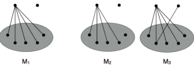
Briefly speaking, modules describe a character that elements of a module behave exactly the same with respect to the outside of the module in a given structure. In a graph, module is defined as a set of vertices that have the same set of neighborhood outside of the module. Precisely, for an undirected graph G = (V, E), a module M _{✓ V (G) satisfies: 8x, y 2 M, N(x) \ M = N(y) \ M, where N(v) denotes the}

(12)

neighborhood of v. In other words, M ✓ V (G) is a module if and only if for all u2 V (G) \ M, either u adjacent to all elements of M or no element of M. Given a subset of vertices C 2 V (G), if there exists u 2 V (G) \ C, and x, y 2 C, such that ux2 E(G) but uy /2 E(G) then u is called a splitter for C.

Figure 1.1: M1 (vertices in the circle) is a module, while M2and M3are not.

Then we introduce the modular decomposition. A strong module is a module that does not overlap with other modules, here we say two non-empty sets A and B overlapif A \ B 6= ;, A \ B 6= ;, and B \ A 6= ;.

Definition 1.2.1. A modular decomposition tree is defined as follows [13]: (a) tree nodes are strong modules;

(b) parent relation is the containment relation of sets represented by tree nodes; (c) each internal nodes is labeled as

• complete if the union of any subset of its children is a module;

• prime if each of its children is a module while no other union of a proper subset of its children is a module.

If a node has only two children, to define this node to be prime or complete is equivalent, we take the convention here that a node has only two children is complete. We give an example of a graph with its modular decomposition tree1 _:

Figure 1.2: Left : A graph with its strong modules grouped. Right: The corre-sponding modular decomposition tree.

(13)

From a series of theorems of partitive family and decomposition [41, 19] that we will present in Chapter 2, it is well-known that the family of modules in a graph corresponds to an unique decomposition tree, and modular decomposition is the procedure to build this decomposition tree.

Modular decomposition in graphs derives several parameters and graph classes to measure the structure of a graph. For example, a graph is totally decomposable (or cograph, P4-free graph) if there is no prime node in the decomposition tree. Cographs

form a well studied graph class where many classical NP -hard problems such as maximum clique, maximum independent set, Hamiltonicity become tractable [25]. Modular decomposition has been used in fixed parameter tractable (FPT) algorithms studies, like Cluster editing [47] or modular width, a graph parameter defined with a similar decomposition procedure following the idea of modular decomposition [40]. The algorithm for modular decomposition is the basic building-block for above applications, and for graphs, it is known to have linear-time algorithms to compute a modular decomposition tree [47, 87].

Besides the study of modules in discrete structures, study of modules have ap-peared recently in networks in social sciences [83], and biology [35, 34], where a module is considered as a regularity or a community that has to be detected and understood.

1.2.2 Generalization of Modules

We consider here generalizing the idea of modules and modular decomposition in order to help characterize and analyze more structures in organized data. For this purpose, we are trying to find out these questions:

• How could we generalize the definition? What structures they characterize? • Are these generalizations well-defined? (i.e. lead to an unique decomposition?) • Could we compute generalized modular decomposition eﬃciently? What is

the time complexity?

We then present the basic elements that decide these questions.

Partitive. Partitive is the essential property required by a valid definition for generalization of modules, because it leads to the unique decomposition. A family of subsets F over a ground set V is partitive if it satisfies the following properties [19]:

(i) ;, V and all singletons {x} for x 2 V belong to F.

(ii) 8A, B 2 F that overlap, A \ B, A [ B, A \ B and A B 2 F. ( denote the symmetric diﬀerence operation)

From [19], every partitive family has a unique decomposition tree. In our work, it’s essential to check if the generalizations are partitive.

(14)

Decomposition algorithm. If the definition is valid, then we turn to the question that if there exists an eﬃcient algorithm for decomposition. Here the algorithm takes the input (in our work it is a graph or a hypergraph), and outputs a tree-structure such that every node is a strong module w.r.t. the definition, and is labelled with either “prime” or “complete” (indicating the prime/complete node in Definition 1.2.1).

Compared to other works in this thesis, here the decomposition algorithm runs in the classical and centralized scenario and the eﬃciency is measured by time com-plexity, where we’d like to have polynomial-time algorithm. Note that even if the family has a unique decomposition tree, the unique decomposition theorem does not guarantee that the decomposition tree could be found in polynomial time, so we need to look into the definition for each generalization.

1.2.3 Related works

For graphs, the only known valid generalization is for module in directed graphs [70], they obtained a linear-time algorithm for modular decomposition in directed graphs.

For hypergraphs, we found three variations of modules: the standard modules [73], the k-subset modules [13] and the Courcelle’s modules [26], each one of them leads to a unique decomposition. Only Courcelle’s module is known to have linear-time decomposition algorithm [18]. For the standard module, the only known previ-ous work is the existence of a polynomial time decomposition algorithm for clutters (a class of hypergraphs) based on its O(n4_m3₎ _{modular closure algorithm [74]. For}

k-subset module, the best known algorithm is not polynomial w.r.t. n and m, and is in O(n3k 5₎_{time [13] where k denotes the maximal size of an edge.}

1.2.4 Outline of Our Work

For graphs, we have looked at ✏-module and ✏-splitter module for graphs, and ob-tained negative results of them. For hypergraphs, we developed O(n3_{· l) algorithms}

for the standard module and the k-subset module, improving the previous known O(n4_m3₎ _{algorithm in [74] and O(n}3k 5₎ _{algorithm in [13] respectively. Note that}

the results for k-subset module also conclude the decomposition of k-subset module in hypargraphs is in P .

Generalization in graphs. In graphs, we consider two generalizations: ✏-module and ✏-splitter module, ✏-module generalizes graph modules in tolerating ✏ edges of errors per node outside the ✏-module (not ✏ errors per module), while ✏-splitter module tolerates errors on nodes.

Definition 1.2.2. A subset M ✓ V (G) is an ✏-module if 8x 2 V (G) \ M, either

|M \ N(x)|  ✏ or |M \ N(x)| |M| ✏

Definition 1.2.3. A subset M ✓ V (G) is an ✏-splitter module if there are at most ✏ splitters in V (G) \ M.

(15)

We conclude in Chapter 2 that these two definitions are not partitive and one-step of parallel decomposition for ✏-module with ✏ = 1 is NP-hard.

Generalization in hypergraphs. We found in the literature three variations of modules defined in the hypergarphs or similar structures: the (we-called) standard modules defined in [73], the k-subset modules defined in [13] and the Courcelle’s modules defined in [26]. And we list these three diﬀerent definitions here:

Definition 1.2.4. (standard hypergraph module [74, 73]) Given a hypergraph H, a standard module M ✓ V (H) satisfies: 8A, B 2 E(H) s.t. A \ M 6= ;, B_{\ M 6= ; then (A \ M) [ (B \ M) 2 E(H).}

Definition 1.2.5.(k-subset module [13]) Given a hypergraph H, we call k-subset module M ✓ V (H) satisfies: 8A, B ✓ V (H) s.t. 2  |A|, |B|  k and A \ M 6= ;, B_{\ M 6= ; and A \ M = B \ M 6= ; then A 2 E(H) , B 2 E(H).}

Definition 1.2.6. (Courcelle’s module [26]) Given a hypergraph H, we call Courcelle’s module a subset M ✓ V (H) that satisfies 8A 2 E(H), A \ M = ; or A_{\ M = ;, or M \ A = ;.}

In Chapter 2 we will see that each of these three diﬀerent definitions of module leads to a unique decomposition theorem via the properities of partitive families [19].

We then developed a general algorithmic scheme following the idea of a work of modular decomposition for graphs [52], generalize it for standard hypergraph module and k-subset module. The algorithmic scheme assumes we know comput-ing a function Minmodule({x, y}), 8x, y 2 V , that is, the smallest module that contains vertices x and y, and builds the decomposition tree based on calls to M inmodule(_{{x, y}), 8x, y 2 V .}

Theorem 1.2.1.For every partitive family F over a ground set V , its decomposition tree can be computed using O(|V |2₎ _{calls to Minmodule({x, y}), with x, y 2 V .}

So if computing the function Minmodule({x, y}) can be done in O(p(n))time, then the computation of the decomposition tree can be done in O(n2_{· p(n)). We}

then showed that for standard hypergraph module and k-subset module, we can compute Minmodule({x, y}) both in O(n · l) time, where l is l the sum of the size of the edges.

Lemma 1.2.1. For a simple hypergraph H and A ( V (H), there is an algorithm computes the minimal standard module that contains A in O(n · l) time.

Lemma 1.2.2. For a simple hypergraph H and A ( V (H), there is an algorithm, s.t. for any input integer k  |V (H)| it can compute the minimal k-subset module that contains A in O(n · l) time.

Combine these results, we get O(n3_{· l) algorithms for modular decomposition of}

standard module and k-subset module.

Theorem 1.2.2. For a simple hypergraph H, the modular decomposition for stan-dard module and k-subset module could be computed in O(n3_{· l) time.}

(16)

1.2.5 Contribution

We studied the generalization of modular decomposition, including two for graphs and three variations of definition of modules for hypergraphs.

For ✏-module in graphs, we showed that ✏-module and ✏-splitter module are not partitive and one-step parallel decomposition of ✏-module with ✏ = 1 is NP-hard.

For hypergraphs,

1. We found three variations of modules in the literature: the standard modules [73], the k-subset modules [13] and the Courcelle’s modules [26], each one of them leads to a unique decomposition.

2. We developed a general algorithmic scheme following the idea in [52], to com-pute the decomposition tree of a partitive family on ground set V using O(|V |2₎

calls to Minmodule({x, y}), with x, y 2 V .

3. We proved that Minmodule({x, y}) of standard module and k-subset module could be computed both in O(n·l) time, which result in O(n3_{· l) algorithm for}

modular decomposition of standard module and k-subset module, improving the previous result based on a O(n4_m3₎ _{algorithm [74] and O(n}3k 5₎

algo-rithm [13] respectively, also conclude the decomposition of k-subset module in hypergraphs is in P .

1.3 Generalized Binary Search Problem

In large graph applications, it happens quite often that we are usually operating with distributively stored information, the access of datas is realized by querying to a storage that we call them oracles. One factor influencing the eﬃciency is the time of queries, for example, when we request for information from a remote server, there will be time delay for receiving the responses. Here we study search problem, a kind of modelization for information exploration.

1.3.1 Search Problem

The search problem is to locate a “hidden” target node in a graph by asking queries to a given oracle. Assume we have a graph G = (V, E, w) with weight function w : V ! R+ and a target node x, each time we selects a vertex v in the graph, ask

to the oracle the partial information of x related to vertex v, which we call a “query”, and after time w(v), we receive the information of x, and w(v) is regarded as the cost of the query.

Many applications have the similar oracles that provide partial information, for example, locating an element in tree-organized data like XML, oracles may only reply “if the target is a child of node v?” for a given v. Also, in classification problem, where every element has some attributes, and we want to classify them into several classes, we are not able to know which class the element belongs to at a single step, but we perform tests as “is the first attribute of the element satisfies the v-th class?” and so on. More over, in these applications, the cost of query may not

(17)

be restricted to the real response time, but also could be the computation resource consumption, etc.

Depend on diﬀerent query model, ways to design search strategies are diﬀerent. We present firstly the formalization of search strategies, then our generalized binary search model.

Search strategy. A search strategy A for a graph G = (V, E, w) is an adap-tive algorithm which defines successive queries to the graph, based on responses to previous queries, with the objective of locating the target vertex in a finite number of steps.

A search strategy could be described by QA(G, x)the time-ordering (sequence) of

queries performed by strategy A on graph G to find a target vertex x, with QA,i(G, x)

denoting the i-th queried vertex in this time ordering, 1  i  |QA(G, x)|.

Cost of a strategy. We denote by COSTA(T, x) =P|Qi=1A(T,x)|w(QA,i(T, x))the sum

of weights of all vertices queried by A with x being the target node, i.e., the time after which A finishes. Let

COSTA(T ) = max_x2V COSTA(T, x)

be the cost of A. We define the cost of T to be

OPT(T ) = min{COSTA(T ) A is a search strategy for T }.

The goal is to design a search strategy that locates the target node and minimizes the search time in the worst case. We say that a search strategy is optimal for T if its cost equals OPT(T ). For given T , we say that a search strategy A is a (1 + ")-approximationof the optimal solution if COSTA(T ) (1 + ")OPT(T ).

1.3.2 Generalized Binary Search

The generalized binary search model, as its name suggests, is generalized from the binary search: considering searching for an element in a sorted array, this could be seen as a problem of searching for a target node in a path, each query selects a node, and the oracle replies which ‘side’ (or sub-path) of the queried node the target node belongs to. When we generalize the structure of path to graphs, this coincides with the generalized binary search model. We give a precise description here.

Generalized Binary Search model. In generalized binary search model, each query selects a node v in the graph and after the time w(v), the oracle gives a reply: the reply is either true which implies that v is the target node and thus the search terminates or it returns a neighbor u of v which lies closer to the target x than v ( equivalent to a neighbor that belongs to the shortest path between x and v). In a general graph, this node may not be unique and we assume that the oracle may reply any one of these nodes. If the graph is a tree, such a neighbor u

(18)

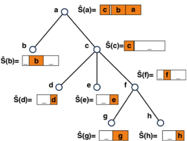
Query e c d e f g _h a b Reply : c Query c c d e f g _h a b Reply : f Query g c d e f g _h a b Reply : f Query : f c d e f g _h a b Reply : true Number of Queries:

Total of 4 queries to locate target: e, c, g, f Figure 1.3: An example of searching a target node (assumed f) in a tree with a generalized binary search query model.

is unique and is equivalently described as the unique neighbor of v belonging to the same connected component of T \ {v} as x.

By tuning several settings, there are variations of generalized binary search model, we list here the main variations: reliable/unreliable oracle, edge/mode query oracle.

Variation: reliable/unreliable oracles. The oracle is reliable if it always replies the correct information to the query, but there are also studies on oracles that doesn’t always reply correct answers. The generalized binary search with an oracle whose answer to a query is correct with some probability p > 1

2 is studied in [8, 37, 38, 53].

And a model in which a fixed number of queries can be answered incorrectly during a binary search is studied in [79]. The model with an adversarial error rate bounded by a constant r  1/2 is studied in [32].

Variation: edge/vertex queries. We could also consider the version that each query is on an edge, and the oracle reply one of the incident vertex that is closer to the target. In fact, the edge-query variant can be reduced to vertex-query model by first assigning a ‘large’ weight to each vertex of G (for example, one plus the sum of the weights of all edges in the graph) and then subdivide each edge e of G giving to the new node the weight of the original edge, w(e). So the vertex-query model is

(19)

more general than the edge-query model. However, in history, the edge variant of trees has been more studied [60, 72, 29, 28, 24, 23].

In the following of this thesis, when we say “search problem”, we assume that we are restricting to the search problem with classical (reliable, node-query) generalized binary search model, except otherwise stated.

Different graph types. There are also many studies on different type of graphs on edge or vertex query model. From a structural aspect, there are mainly on paths [23], trees [76, 81, 31], directed or undirected general graphs [37] and partial orders [17, 29, 76]. From an quantitive aspect, there is difference between weighted or unweighted graph (meaning the uniform or non-uniform query costs), the difference is discussed in some of the works listed, and we will present it more detailed nextly in Section 1.3.3.

1.3.3 Related Works

In this thesis, we study the generalized binary search with reliable oracles and vertex-queries. As the existence of reduction of edge-query to vertex-query, we don’t need to state for edge-query model and the results for vertex-query naturally apply for edge-query model.

We list here the complexity results for diﬀerent type of graphs.

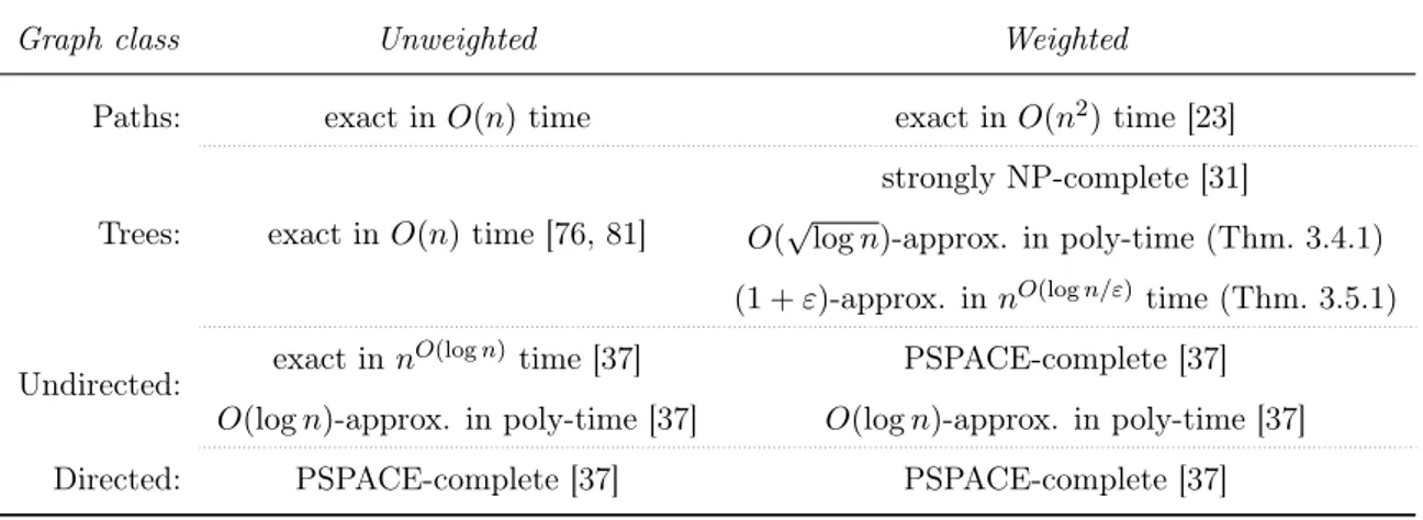
Table 1.1: Computational complexity of the search problem in diﬀerent graph classes, including our results for weighted trees. Completeness results refer to the decision version of the problem.

Graph class Unweighted Weighted

Paths: exact in O(n) time exact in O(n2₎_{time [23]}

Trees: exact in O(n) time [76, 81] strongly NP-complete [31] Undirected: exact in n

O(log n)_{time [37]} _{PSPACE-complete [37]}

O(log n)-approx. in poly-time [37] O(log n)-approx. in poly-time [37]

Directed: PSPACE-complete [37] PSPACE-complete [37]

An optimal search strategy can be computed in linear-time for an unweighted tree [76, 81]. The number of queries performed in the worst case may vary from being constant (for a star one query is enough) to being at most log2n for any tree

[76] (by always querying a node that halves the search space). Several following results have been obtained in [37]. First, it turns out that log2nqueries are always

suﬃcient for general simple graphs and this implies a O(mlog2nn2log n)-time optimal

algorithm for arbitrary graphs. The algorithm which performs log2n queries also

(20)

problem. On the other hand, it has been proven that optimal algorithm with a run-ning time of O(no(log n)₎ _{is in contradiction with the Exponential-Time-Hypothesis,}

and for " > 0, O(m(1 ") log n₎_{is in contradiction with the Strong}

Exponential-Time-Hypothesis. When non-uniform query times are considered, the problem becomes PSPACE-complete. Also, a generalization to directed graphs also turns out to be PSPACE-complete.

1.3.4 Outline of Our Work

We study the generalized binary search problem in weighted trees. Given a node-weighted rooted tree T = (V, E, w) with weight function w : V ! R+, we would like

to have good strategies to find the unknown target node x with generalized binary search oracle. As designing an optimal strategy for a weighted tree search instance is known to be strongly NP-hard [31], we aim at computing an approximation of the optimal strategy.

In order to apply classical approximation techniques to this problem, following the idea in [28], we model in Section 3.3.2 any search strategy as a consistent schedule, where each node is associated with a job that has a fixed processing time set to the weight of node, and jobs need to satisfy the consistent constraints. We then see that we have a description similar to scheduling problems, but with non-classical constraints. With this model, we are able to apply techniques in ap-proximation algorithm for scheduling problems as rounding [88].

In Section 3.4.1 and 3.4.2, we apply rounding techniques to both the cost func-tion and starting times of the jobs in a schedule, and finally created the aligned schedule, such that any optimal strategy could be turned into an aligned consis-tent schedule whose modified cost function is a (1+")-approximation of the optimal strategy. Then if we could enumerate all aligned consistent schedules, we are able to obtain the optimal aligned schedule, and a (1 + ")-approximation of cost of the optimal strategy.

In section 3.4.3, we propose a dynamic programming algorithm to enumerate aligned consistent schedules, and runs in quasi-polynomial time. Then in sec-tion 3.4.4, we explain how to extract the search strategy from the optimal aligned consistent schedule, together with 3.4.5 this procedure adds no more than "OPT(T ) to the cost, so the obtained search strategy is a (1+")-approximation of the optimal, and our algorithm computing the strategy runs in quasi-polynomial time, thus the QPTAS of the generalized binary search problem in weighted trees, and we get our first theorem on generalized binary search problem in weighted trees:

Theorem 1.3.1. There exists an algorithm running in nO(log n_"2 ) time, providing a

(1 + ")-approximation solution to the generalized binary search problem in weighted trees.

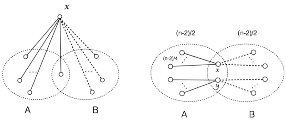
Based on our QPTAS, we could also build a polynomial time approximation al-gorithm. In Section 3.5, following the general idea from [24], we apply a recursively partition method, whose objective is to partition the tree into small subtrees, such that the sizes of these subtrees are small enough then we could solve the problem

(21)

on these subtrees with our QPTAS in polynomial time with respect to |T |, so com-bining solutions of these subtrees, we get a O(plog n)-approximation algorithm in polynomial time:

Theorem 1.3.2. There is a O(plog n)-approximation polynomial time algorithm for the generalized binary search problem in weighted trees.

1.3.5 Contribution

We work on the generalized binary search problem in weighted trees, show that: 1. The problem admits a quasi-polynomial time approximation scheme: for any

" > 0, there exists a (1+")-approximation strategy with a computation time of nO(log n/"2₎

. Thus, the problem is not APX-hard, unless NP ✓ DT IME(nO(log n)_).

2. By applying a generic reduction, we obtain as a corollary that the studied problem admits a polynomial-time O(plog n)-approximation. This improves previous ˆO(log n)-approximation approaches, where the ˆO-notation disregards O(poly log log n)-factors.

1.4 Pure-LOCAL Model and Max-flow Problem

Here we present the model we work on in distributed computing environment, and build the approximation algorithm for maximum s t flow problem on it.

We first introduce the basic settings in distributed computing and present our model.

Distributed Computing In the classical configuration of distributed comput-ing, machines are organized into a graph G = (V, E), where each vertex (or node) has an unique identifier and represents a machine that has computation ability and resources, and each edge (u, v) 2 E represents a communication link between ma-chines u, v, meaning u and v could send messages (a number of bits) to each other directly. We could assume here that the graph is undirected, connected and simple. We call u, v are neighbors if (u, v) 2 E, and denote N(u) as all the neighbors of u2 V .

Every vertex and edge could be associated with a label, the state of the labels of all vertices and edges constitutes a configuration. In distributed computing, an inputis a configuration set to the graph, and an output is the configuration after some operations (or the execution of an algorithm) on the graph.

An algorithm here is called a distributed algorithm, compared to classical al-gorithms, here we could have two extra operations, send and receive messages. A send operation could send messages to its selected neighbors (could be any one, some or all). A receive operation, symmetrically, could receive messages from its selected neighbors, but only receive in success if the selected neighbor had sent to it.

In the study of distributed algorithms, being diﬀerent than some other disciplines of distributed computing, we are not focusing on the synchronization problem. Here

(22)

we assume all the machines are synchronized with rounds, in a round, each machine can receive messages from its neighbors, do its local computation, and send messages to its neighbors.

The complexity measure of a distributed algorithm is thus the number of rounds from getting the input to get the output. And depend on diﬀerent models, there might be other measure or constraints on computing resources or graph structures, in the next section we present our model.

1.4.1 Pure-LOCAL Model

We consider a model with limited memory per node, specifically every node can only store a constant number of variables per degree:

Pure-LOCAL. We define our Pure-LOCAL model as following: (i) The network is represented as a graph G = (V, E), where edges represent the bidirectional com-munication link, and each node only knows and can communicate with its neighbors. (ii) Communications are synchronized, this means each node can proceed one receive and one send operation from/to each neighbor during one round, and we measure the time complexity by number of rounds. (iii) A node can only store and one send operation could only send a constant number of variables for each of its neighbors.

If the degree of a vertex u is deg(u), then it implies the node could store O(deg(u)) variables. Here if we assume real variables are stored in constant number of bits, it implies a limited size of memory of O( log n) bits per node and O(log n) message size, where is the maximum degree of all nodes in the graph.

The motivation to study this model is to impose the memory eﬃciency and local-ity of computation. The classical LOCAL model [63, 77] does not bound computing power per node and the CONGEST model [77] put a restriction on LOCAL model with O(log n) bits of message size, but no constraints on computing resource per node. These two classical model both admit a general framework of gathering all the information on one node and launch computations on this node, and this kind of framework is applied in a lot of scenes of algorithm design on LOCAL/CONGEST model.

Although the two models support well the study on locality and in situations that the computing power of a single machine is not an important concern than communication costs, the assumption of unbounded computing power on machines is less realistic in some scenarios. For example, in the network of low energy devices, like wearable or medical devices, smart domestic systems, the execution of complex or high complexity algorithms could be diﬃcult. Another example is the natural algorithms, which studies the algorithms on biological objects, as animals, microbes and chemicals, it seems less natural to assume their behaviors are following complex algorithmic rules.

Our model could be seen as a classical CONGEST model with a limit of memory size on each node, and naturally being more constrained than CONGEST model. This is a memory-eﬃcient assumption but also reflects the requirement of simplicity of algorithm on each machine.

(23)

In our work, we study the algorithm design for maximum s t flow problem on this model.

1.4.2 Maximum s t Flow Problem

The maximum s t flow problem is well known in combinatorial optimization [82, 1] and has many application in logistics, transportation and industry engineering [2], and its dual problem, the minimum s t cut, has also a application of the famous graph cut method [16] which receives recent attentions in image segmentations, and is implemented by solving the maximum s t flow problem.

The problem could be stated as following:

Let G = (V, E) be an undirected graph, with n vertices and m edges, among which there are two special vertices, a source s and a sink t. Every edge is assigned with a positive integral capacity Ue2 Z+. Let A be the adjacency matrix of G

Definition 1.4.1.An s-t flow is a function f : E ! R obeying the flow-conservation constraints

X

e2N(v)

f (e) = 0, for all v 2 V \ {s, t}

The value of flow |f| is defined by |f| :=Pe2N(s)f (e) and is equal to

P

e2N(t)f (e)

by flow-conservation.

Here Ue is the edge capacity and we assume that is polynomial w.r.t. n. An

s-t flow is feasible for capacities Ue if 8e 2 E, |f(e)|  Ue. The maximum s-t flow

problem is to find a feasible s-t flow with maximum value.

In centralized settings, many polynomial combinatorial algorithms have been proposed to solve maximum s t flow problem in history, including the Ford-Fulkerson algorithm [39], Edmonds-Karp algorithm [36], push-relabel algorithm [44], etc. And recently, another series of study is raised on using continuous optimization method to compute (1 + ") approximation of maximum s t flow [20, 61, 68] their basic framework is to regard the maximum s t flow problem as an optimization problem defined by a Laplacian system (which is equivalent to the description of the electrical flow in circuits) and optimize with a Laplacian solver [55], where two main optimization techniques are adopted to approximate the optimal solution: the multiplicative weights update method [4, 20] and gradient descent based method [61]. Our work is based on one of these works [20] based on multiplicative weights update method and electrical flow and we will present basics in later sections.

Solving this problem in classical distributed configurations has also been studied, and algorithms are basically designed by implementing one or a combination of classical centralized algorithms to an distributed version. The push-relabel algorithm [44] could be naturally implemented in Pure-LOCAL model and runs in O(V2_E)

time. In [42] authors proposed an (1+o(1))-approximation algorithm on CONGEST model in (D +pn)no(1) _{rounds, which their method depend on gradient descent}

(24)

Although the push-relabel algorithm could fits the local computation, we are now interested in the question that whether non-combinatorial algorithms for Max-flow problem could be implemented in Pure-LOCAL model. And we study the algorithm of [20] by Christiano, Kelner, Mądry, Spielman and Teng. The reason to study this category of algorithms in Pure-LOCAL model is that the general optimization techniques they use could be applied to many other problems, for example, the work on Physarum dynamics [5] also suggests a similar procedure combining electrical flow and re-weighting, and we wish that our method could also be applied to implementing these procedures in Pure-LOCAL model.

1.4.3 Approximating Max-flow by Multiplicative Weights

Up-date

An algorithm approximating Max-flow by solving electrical flow with weights updat-ing is presented in [20]. Intuitively, one can think the settupdat-ing of Max-flow is quite similar to electrical flow, but with a diﬀerent objective function. Can we adjust resistances in an electrical circuit such that the electrical flow tends to the max-flow in this graph?

In [20], Mądry et al utilize the electrical flow connection and iteratively choose resistances in an constant current source electrical network, such that the average of electrical flow they get among all rounds tends to the max-flow if the source flow value is close to the max-flow value. In fact they are considering the decision problem of approximating maximum s t flow problem.

Decision problem of approximating Max-flow problem. The decision

prob-lem of (1+") approximation of Max-flow is that, given a graph G = (V, E) with edge capacity Ue, e 2 E and a value F , we’d like to check if F exceed the (1 + O(")) of

the maximum flow and otherwise returns an s t flow ¯f such that | ¯f| (1 O("))F and for every e 2 E, ¯fe Ue.

If there is an algorithm solves the (1 + ") decision problem of Max-flow, we could compute a (1+O(")) approximation of the Max-flow by launching a binary search on value F , i.e. set F = 1 and run the algorithm, then multiply F by (1 + ") each time until there returned an “no”. Then the previous value is a (1 + O(")) approximation, and this binary search procedure brings an log(1+")Fmaxfactor to the running time.

Multiplicative weight update method for Max-flow. In [20], Mądry et al

(25)

w(0) e = 1,8e 2 E r(t)_e = 1 U2 e (w(t)_e +" w (t) 1 3m ) f(t)

e =electrical flow induced by r(t) and F

cong(f_e(t)) = f (t) e Ue w(t) e = w(t 1)e ✓ 1 +" ⇢conge(f (t 1)₎ ◆ (1.1)

Where Ue is the edge capacity and conge(f ) = _Ufe_e is the congestion of an edge,

⇢ is a parameter. They showed if F is a (1 + O(")) approximation of Max-flow, then an (1 ") factor of the average of these electrical flow computed in all rounds satisfy the edge capacity constraints and is an (1 + O(")) approximation of Max-flow, and can return “NO” if F not. In fact, they also show that the computation of the electrical flow does not need to be exactly, i.e. an approximate solution of the electrical network is enough.

Challenges of implementation in Pure-LOCAL model. To implement the

Algorithm 1.1 in Pure-LOCAL model, there are two main challenges: 1. How to compute kw(t)k1

m the average of weights ? It’s not trivial because

w(t)

1 is a global quantity and is changing between iterations.

2. How to compute the electrical flow induced by r(t) _{and F ? Computing an}

electrical flow could be reduced to solve a Laplacian system as we will present in Section 4.2.1, but there is no known general Laplacian solver in Pure-LOCAL model with weight-updating.

1.4.4 Outline of Our Work

We study the design of algorithm in [20], by Mądry et al in Pure-LOCAL model. As in the above section, we have two challenges in turning Mądry et al’s algorithm in Pure-LOCAL model: estimating the average of weights and approximating the electrical flow. We propose to solve these two challenges by matrix computations from the idea of random walk.

We are going to show that, the simple random walk in a graph could ap-proximate the average of weights, and the weighted random walk with edge conductancescould approximate the flow of an electrical network. To handle the issue that weights are changing with iterations, we design the “slow down” parame-ters, such that the weights do not change too much before we get an approximation that has an error small enough of the quantities we need.

In Section 4.2.2 we present the connection of Max-flow problem and electrical flow and the idea of approximating Max-flow by optimization technique and solving electrical networks. In Section 4.2.1 we present the preliminary connection of elec-trical flow and graph Laplacian that compute an elecelec-trical flow could be reduced to

(26)

solve a Laplacian system. In Section 4.2.3 we introduce the basics of random walk, and the idea to approximate intended quantities in our algorithm.

In Section 4.3 we describe our algorithm both in dynamical system way and Pure-LOCAL distributed algorithm way. In Section 4.4.2 and Section 4.4.1 we show that the re-weighting process in our algorithm provide a vector approximating (1 + O(")) Max-flow if there could be an (1 + ")-energe approximation of electrical flow. In Section 4.4.3 we show that our algorithm build an (1 + ")-energe approximation of electrical flow.

We need to precise that, our approximation algorithm in Pure-LOCAL model does not provide a solution to the original decision problem but a weaker version:

Weaker decision problem of Max-flow approximation. Our algorithm solve a weaker decision problem of (1 + ") approximation of Max-flow: given a graph G = (V, E)with edge capacity Ue, e 2 E and a value F , if F does not exceed the

maximum flow, we will return “YES” . And if we return “NO” then F must exceed the maximum flow. More precisely, let F⇤_{be the max-flow value, we will compute a}

vec-tor ¯f, such that if F  F⇤_{then cong}_e_{( ¯}_{f )}_{ 1, and if cong}_e_{( ¯}_{f ) >} (1+")2

(1 ")2 then F > F⇤.

This weakness compared to the centralized algorithm in [20], is that the ap-proximated electrical flow that our algorithm produces may have an error on flow-conservation constraints, thus we are not able to ensure the vector ¯f is an s t flow and lead to this one-side result.

1.4.5 Contribution

We studied the implementation of an multiplicative weights update algorithm ap-proximating Max-flow problem in Pure-LOCAL model.

1. We design the way in Pure-LOCAL model to approximate the global quantity of average weight in a weight-varying iterative algorithm.

2. We implement in Pure-LOCAL model the computation to solving an electrical network with resistances changing in iterations. As we know, this is the first algorithm approximating the electrical flow in a weight-varying environment. 3. We show that our algorithm solves a weaker version of Max-flow approximation

decision problem in polynomial time.

Perspective We’d like to apply our method to implement other weight-update based algorithm in Pure-LOCAL model, i.e. the Physarum dynamics [5] that com-putes the shortest path, etc.

(27)

1.5 Publications during PhD

• Michel Habib, Fabien de Montgolfier, Lalla Mouatadid, Mengchuan Zou: A General Algorithmic Scheme for Modular Decompositions of Hypergraphs and Applications.

International Workshop on Combinatorial Algorithms (IWOCA) 2019, invited to a special issue of Journal Theory of Computing Systems

• Michel Habib, Lalla Mouatadid, Mengchuan Zou: Approximating Modular Decomposition is Hard.

Accepted to The International Conference on Algorithms and Discrete Applied Mathematics (CALDAM) 2020.

The second publication here presents also some positive results of enumerating all minimal "-modules, which are not included in this thesis.

• Dariusz Dereniowski, Adrian Kosowski, Przemyslaw Uznanski, Mengchuan Zou: Approximation Strategies for Generalized Binary Search in Weighted Trees. International Colloquium on Automata, Languages, and Programming (ICALP), 2017

(28)

Chapter 2 Generalization of Modular

Decompositions

This chapter considers the generalization of modular decomposition and its eﬃcient algorithms. We study two type of generalizations: (1)Modular decomposition in hypergraphs; (2)Allowing errors in modules of graphs. We present both positive and negative (hardness) results.

We first present the hypergraph modular decomposition. In the literature we find three diﬀerent definitions of modules, namely: the standard one [73], the k-subset modules [13] and the Courcelle’s one [26]. They all lead to partitive families, and thus each accepts an unique decomposition tree. For Courcelle’s module an linear-time decomposition algorithm is already known [18], and we study designing eﬃcient algorithms for the standard and the k-subset modular decomposition of hypergraphs.

When allowing errors in graph modules, we look at two definitions: ✏-module and ✏-splitter module, we conclude that they are not partitive thus do not satisfy the condition of the unique modular decomposition theorem. More over, testing of one-step parallel decomposition ✏-module for ✏ = 1 is already NP-hard.

2.1 Preliminaries and Definitions

2.1.1 Classical Modular Decomposition

Let G be a simple, loop-free, undirected graph, with vertex set V (G) and edge set E(G), n = |V (G)| and m = |E(G)| are the number of vertices and edges of G re-spectively. N(v) denotes the neighbourhood of v and N(v) the non-neighbourhood, this notation could also be generalized to set of vertices, i.e. N(X) (resp. N(X)) , for X ✓ V (G), are vertices who have (resp. haven’t) a neighbour in X.

Definition 2.1.1. For an undirected graph G, M ✓ V (G) is a module if and only if: 8x, y 2 M, N(x) \ M = N(y) \ M.

In other words, V (G) \ M is partitioned into X, Y such that there is a complete bipartite between M and X, and no edge between M and Y . For convenience let

(29)

us denote X (resp. Y ) by N(M) (resp. N(M)). For x, y 2 V , we call them false-twinsif N(x) = N(y) and true-twins if N(x) [ {x} = N(y) [ {y}. It’s easy to see that all vertices within a module are at least false twins.

Here we give an example of a graph with a partition by strong modules. 1

Figure 2.1: Strong modules in G are: {1}, {2,3,4},{5},{6,7}, {8,9,10,11} A single vertex {v} and V are always modules, and called trivial modules. A graph that only has trivial modules as induced subgraphs is called a prime graph. Two non-empty sets A and B overlap if A \ B 6= ;, A \ B 6= ;, and B \ A 6= ;. A strong moduleis a module that does not overlap with other modules.

Definition 2.1.2. A modular decomposition tree is defined as follows [13]: (a) tree nodes are strong modules;

(b) parent relation is the containment relation of tree nodes;

(c) each internal node with only two children is labeled as complete and each other internal node is labeled as

• complete if the union of any subset of its children is a module;

• prime if each of its children is a module while no other union of a proper subset of its children is a module.

In the case of graphs, in fact complete nodes could also be distinguished by two types of operations: parallel (disjoint union) and series (connect every pair of nodes in disjoint sets X and Y ).

By the Modular Decomposition Theorem [41], any graph accepts a unique mod-ular decomposition tree. A graph is totally decomposable if there is no prime node in the decomposition tree. Totally decomposable graphs with respect to mod-ular decomposition are also known as cographs in the literatture, or P4-free graphs.

(30)

Cographs form a well studied graph class where many classical NP -hard prob-lems such as maximum clique, maximum independent set, Hamiltonicity become tractable, see for instance [25].

Sets that do not overlap are said to be orthogonal, which is denoted by A ? B. Let F be a family of subsets of a ground set V . A set S 2 F is called strong if 8S0 _{6= S 2 F : S ? S}0_.

Definition 2.1.3. [19] A family of subsets F over a ground set V is partitive if it satisfies the following properties:

(i) ;, V and all singletons {x} for x 2 V belong to F.

(ii) 8A, B 2 F that overlap, A \ B, A [ B, A \ B and A B 2 F, here denote the symmetric diﬀerence operation.

The study on partitive families extends the results of [41], in [19] they show every partitive family admits a unique decomposition tree, with the two types of nodes as in Definition 2.1.2. In this decomposition tree, every node corresponds to a set of the elements of the ground set V of F, and the leaves of the tree are single elements of V , strong elements of F form a tree ordered by the inclusion relation. For a complete (resp. prime) node, every union of its child nodes (res. no union of its child nodes other than itself) belongs to the partitive family.

The uniqueness of decomposition tree for partitive families provides us the foun-dation to study the generalization of modular decomposition upon families that are partitive.

2.1.2 Hypergraphs

Following Berge’s definition of hypergraphs [9], a hypergraph H over a finite ground set V (H) is made by a family of subsets of V (H), denoted by E(H) such that (i) 8e 2 E(H), e 6= ; and (ii) [e2E(H)e = V (H). We assume here also a hypergraph

admits no empty edge and no isolated vertex.

When analyzing algorithms, we use the standard notations: |V (H)| = n, |E(H)| = mand l = ⌃e2E(H)|e|. For every edge e 2 E(H), we denote by H(e) = {x 2 V (H)

such that x 2 e}, and for every vertex x 2 V (H), we denote by N(x) = {e 2 E(H) such that x 2 H(e)}.

To each hypergraph one can associate a bipartite graph G, namely its incidence bipartite graph, such that: V (G) = V (H) [ E(H) and E(G) = {xe with x 2 V (H) and e 2 E(H) such that x 2 H(e)}.

A hypergraph is simple if all its edges are diﬀerent. In this case E(H) ✓ 2V (H)_.

For a hypergraph H and a subset M ✓ V (H), let H(M) denote the hypergraph induced by M, where V (H(M)) = M and EH(M ) ={e \ M 2 E(H), for e \ M 6= ;}.

Similarly, let HM denote the reduced hypergraph where V (HM) = (V \ M) [ {m})

with m /2 V , and E(HM) = {e 2 E(H) with e \ M = ;} [ {(e \ M) [ {m} with

e2 E(H) and e \ M 6= ;}. By convention in case of multiple occurences of a similar edge, only one edge is kept and so HM is a simple hypergraph.

(31)

2.2 Variant Definitions of Hypergraph Modules

2.2.1 Standard Modules

In the literature three variations of modules defined in the hypergraphs, and we first introduce the one defined in [73] that we called a standard module.

Definition 2.2.1(Hypergraph Module). Given a hypergraph H, a standard mod-ule M ✓ V (H) satisfies: 8A, B 2 E(H) s.t. A \ M 6= ;, B \ M 6= ; then (A\ M) [ (B \ M) 2 E(H).

The reason we name it as standard is that this definition relates to the following hypergraph substitution operation.

Hypergraph substitution: Substitution in general is the action of replacing a vertex v in a graph G by a graph H(V0_{, E}0₎ _{while preserving the same}

nerigh-bourhood properties. To apply this concept to hypergraphs, we use the definition presented in [74, 73]:

Definition 2.2.2. Given two hypergraphs H, H1, and a vertex v 2 V (H) we can

define another hypergraph H0 _{obtained by substituting in H the vertex v by the}

hy-pergraph H1, and denoted by H0 = HvH1 which satisfies V (H0) ={V \ v} [ V (H1),

and E(H0_{) =} _{{e 2 E(H) s.t. v /}_{2 e} [ {f \ v [ e}

1 s.t. f 2 E(H) and v 2 f and

e12 E(H1)}.

Note that even if H, H1 are undirected graphs, the substitution operation may

create edges of size 3, and therefore the resulting hypergraph H0_{is no longer a graph.}

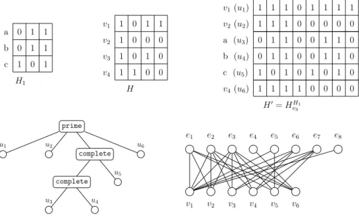
Proposition 2.2.1. The class of simple hypergraphs is closed under substitution. When M is a module of H then H = (HM)H(M )m . On the previous example: let

us take A, B 2 E (resp. 1st _{and 6}th _{columns of H}0_{) then (A \ M) [ B \ M = 2}nd

column of H0 _{and therefore belongs to E.}

Let’s consider the example below where hypergraphs are described using their incidence matrices. In this example, we substitute vertex v3in H by the hypergraph

H1 to create H0:

If M is a module of H then 8e 2 E(HM), the edges of H that strictly contain e

and are not included in M are the same. In other words, all edges in E(HM)behave

the same with respect to the outside, which is an equivalence relation between edges. Proposition 2.2.2. [74] The family of all standard modules of a simple hypergraph H yields a partitive family on |V (H)|.

Proof. Of course every singleton of V (H) is a module and V (H) itself is also a module.

Let us consider two modules A, B that overlap. Using the above definition via an equivalence relation between edges, it is clear that A \ B is also a module. Similarly as there exists at least one edge in EA\B since H is simple, by transitivity of this

(32)

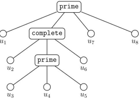
a 0 1 1 b 0 1 1 c 1 0 1 H1 v1 1 0 1 1 v2 1 0 0 0 v3 1 0 1 0 v4 1 1 0 0 H v1(u1) 1 1 1 0 1 1 1 1 v2(u2) 1 1 1 0 0 0 0 0 a (u3) 0 1 1 0 0 1 1 0 b (u4) 0 1 1 0 0 1 1 0 c (u5) 1 0 1 0 1 0 1 0 v4(u6) 1 1 1 1 0 0 0 0 H0_{= H}H1 v3 prime u1 u2 complete complete u3 u4 u5 u6 e1 e2 e3 e4 e5 e6 e7 e8 v1 v2 v3 v4 v5 v6

Figure 2.2: An example of substitution, its decomposition tree, and its incidence bipartite graph. {u3, u4, u5} is a module, but only u3, u4 are false twins in the

incidence bipartite.

A_{\ B the only case to check if the following: F, F}0 _{2 E(H(A \ B)) such that}

F [ C 2 E(H) with C ✓ A \ B. Since B is an module, necessarily F0_{[ C 2 E(H).}

Therefore A \ B is also a module of H.

Similarly, let F 2 E(H(A\B)) such that F [C 2 E(H) with C ✓ A\B. Now if we consider F0_{2 E(H(B \ A)), using the fact that B is a module and C, F}0_{2 E(H(B))}

then F [ F0_{2 E(H). But then since A is a module and F, C 2 E(H(A)) necessarily}

C_{[ F}0_{2 E(H). Thus, A B is a module of H.}

Remark: if we use the following variant definition for hypergraphs :

Given a hypergraph H, a module M ✓ V (H) satisfies: 8A, B 2 E(H) s.t. A_{\ M 6= ;, A \ M 6= ;, B \ M 6= ;, B \ M 6= ; then (A \ M) [ (B \ M) 2 E(H).}

Unfortunately this definition does not lead to a partitive family. Simply because using this definition, any set of size |V | 1 is a module, because any edge overlapping outside connects the same vertex. Then any set of size |V | 2 is a module because it is the intersection of two sets of size |V | 1. By induction we could have that any set is a module if the definition is partitive. However it could not be true. So the intersection property may fail.

Since every partitive family has a unique decomposition tree [19], it follows that the family of the modules of a simple hypergraph admits a uniqueness decomposition theorem and a unique hypermodular decomposition tree.

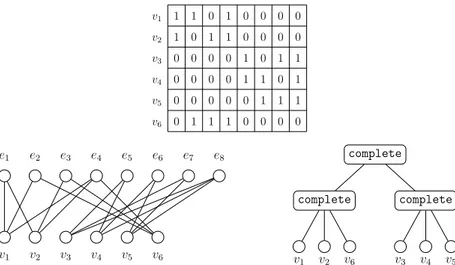
Consider the graph in Figure 2.3 which represents the incidence bipartite of the hypergraph H0 _{constructed in the previous example, together with a renumbering}

(33)

v1 1 1 0 1 0 0 0 0 v2 1 0 1 1 0 0 0 0 v3 0 0 0 0 1 0 1 1 v4 0 0 0 0 1 1 0 1 v5 0 0 0 0 0 1 1 1 v6 0 1 1 1 0 0 0 0 e1 e2 e3 e4 e5 e6 e7 e8 v1 v2 v3 v4 v5 v6 complete complete v1 v2 v6 complete v3 v4 v5

Figure 2.3: A hypergraph H given by its incidence bipartite and its modular de-composition tree

twins in the associated bipartite graph.

Modular decomposition of bipartite graphs just leads to the computation of sets of false twins in the bipartite graphs. So hypergraph modules are not always set of twins of the associated incidence bipartite.

Some authors [10, 11] defined clutters hypergraphs, in which no edge is included into another one. In this case, clutters modules are called committees [10]. Trivial clutters are closed under hypergraph substitution. The committees of a simple clut-ter also yields a partitive family which implies a uniqueness decomposition theorem. From this one can recover a well-known Shapley’s theorem on the modular decom-position of monotone boolean functions. It should be noted however that finding the modular decomposition of a boolean function is NP-hard [12]. It was shown in [15], that computing clutters in linear time would contradict the SETH conjecture.

e1 e2 e3 e4 e5

v1 v2 v3 v4 v5 v6

Figure 2.4: An example of a module M = {v2, v3, v4, v5}

An Application of Standard Module. If we consider that a bipartite graph is the incidence bipartite of some hypergraph then we could apply the modular decomposition of hypergraphs to decompose the bipartite graph, as can be seen in the examples of Figures 2.3, 2.4.