Acknowledgement
First, I would like to express my gratitude to my supervisor, Prof Soraya Benderbous,for her
guidance, and advice she has provided throughout my thesis. I would also like to thank the director of laboratory of INSERM U825, Dr Pierre Celsis, for his support during my PhD.
My thesis work has been performed in collaboration with three laboratories including laboratory of bioorganic and biononorganic of university of paris sud under directory of Dr Hafsa Korri Youssoufi and Dr Helen Dorizon, laboratory of ITODAYS of the university of paris 7 under directory of Prof Souad Ammar Merah, and the laboratory of photonic of Angers under directory of Prof Stephane Chaussedent. I do greatly appreciate for their kind guidance, caring, patience, and providing me with an excellent atmosphere for doing research. I would like to express my deepest gratitude to Prof Francois Sanchez, director of photonic laboratory of Angers, for his warm welcome in the laboratory and his support. Moreover, I am grateful to all the people who have been (and are) working in the lab of photonic and of bioorganic and nonbioorganic, for the great atmosphere and for the helpful attitude.
Finally, I would like to acknowledge with gratitude, the support of all my friends in laboratory Paris sud, Paris 7 and laboratory of photonic of Angers.
i
Contents
SYMBOLS AND ABBREVATIONS ... IV LIST OF FIGURES ... VII LIST OF TABLES ... XI
CHAPTER I: INTRODUCTION ... 3
A. GENERAL INTRODUCTION ... 3
B. OBJECTIVE OF THESIS ... 5
C. THESIS OUTLINE ... 5
CHAPTER II: RELAXATION MECHANISM ... 7
A. BASIC PRINCIPLE OF MRI ... 9
B. RELAXATION TIME ... 10
B.1. Longitudinal relaxation time ... 10
B.2. Transverse relaxation time ... 11
C. PARAMAGNETIC RELAXATION TIME ... 12
C.1. Inner Sphere Proton relaxivity ... 13
C.1.1. Dipolar interaction ... 14
C.1.2. Scalar interaction ... 15
C.1.3. Curie relaxation ... 15
C.2. Second sphere relaxivity ... 16
C.3. Outer sphere relaxivity ... 16
CHAPTER III: LITERATURE REVIEW ... 19
A. TUMOR-TARGETING CONTRAST AGENTS ... 22
A.1. Macrocyclic chelator ... 23
A.1.1. General reviews of Porphyrins ... 25
A.1.2. Synthesis of meso-substituted porphyrin complex ... 26
A.1.3. Electronic absorption Spectrum of porphyrin ... 29
A.2. Application of porphyrin in cancer therapy and imaging ... 32
A.2.1. Photodynamic Therapy ... 32
A.2.2. Fluorescence Imaging ... 33
A.2.3. Magnetic Resonance Imaging ... 34
A.2.4. In-vivo MRI studies of metalloporphyrin ... 36
B. MACROMOLECULAR CONTRAST AGENTS ... 39
B.1. Macromolecular Contrast agents classification ... 41
B.1.1. Block macromolecular contrast agents ... 41
B.1.2. Nano-polymeric macromolecular contrast agents ... 43
B.1.2.1. Chitosan ... 44
B.1.2.2. Protocol of chitosan nanoparticles preparation ... 45
B.1.2.3. Biodegradability, biocompatibility, biodistribution and toxicity of chitosan composites ... 47
B.1.2.4. Chitosan based MRI contrast agents ... 48
B.1.2.5. In-vitro MRI studies of chitosan-based contrast agent ... 48
B.1.2.6. In-vivo MRI studies of chitosan based contrast agents ... 50
C. QUANTUM DOTS ... 51
C.1. Importance of QDs ... 52
C.1.1. Synthesis of QDs ... 53
C.1.2. Ligand exchange approaches towards biologically compatible probes ... 55
ii
C.2.1. Application of Quantum dots as contrast enhancement of MR images ... 57
D. MOLECULAR DYNAMICS SIMULATION ... 58
D.1. Simulation Set-up and procedure ... 60
D.1.1. Molecular dynamic simulation of ZnS and ZnS-doped nanoparticles ... 63
D.1.2. Molecular dynamic simulation of ZnS and ZnS-doped nanoparticles in solution ... 66
CHAPTER IV: MATERIAL AND METHODS ... 69
A. SYNTHESIS OF PORPHYRIN... 71
A.1. Chemical materials ... 71
A.2. Metallation of meso-tetrakis(4-pyridyl)porphyrin with Gadolinium (Gd(TPyP)) ... 71
A.3. Colloid preparation ... 72
A.4. Characterization ... 73
A.4.1. UV-visible spectroscopy ... 73
A.4.2. Matrix assisted laser desorption/ionisation (MALDI)-TOF mass spectrometry ... 73
A.4.3. Fourier transmission infrared spectroscopy ... 73
A.4.4. NMR relaxometry ... 73
A.4.5. Magnetic Resonance Imaging ... 74
B. LOADING OF GD(TPYP) INTO CHITOSAN NANOPARTICLES ... 75
B.1. Chemical Materials ... 75
B.2. Synthesis of Chitosan Nanoparticles (CNs) ... 75
B.3. Preparation of Gd(TPyP) loaded chitosan nanoparticles ... 76
B.4. Characterization of CNs and Gd(TPyP)-CNs ... 77
B.4.1. Dynamic light scattering ... 77
B.4.2. Microscopic imaging of CNs and Gd(TPyP)/CNs ... 78
B.4.3. UV-visible spectroscopy of Gd(TPyP)-CNs ... 78
B.4.4. Fourier transmission infrared spectroscopy ... 78
B.4.5. Inductively coupled plasma mass spectrometry (ICP-MS) ... 78
B.4.6. Magnetic resonance imaging... 78
B.4.7. Determination of entrapment efficiency, loading capacity and yield of Gd(TPyP)/CNs ... 79
C. SYNTHESIS OF ULTRA SMALL MN (II) DOPED ZNS NANOPARTICLES ... 79
C.1. Chemical material ... 79
C.2. Synthesis of Manganese Zinc Sulphide particles ... 80
C.3. Particle Characterization of MnxZn1-xS (x=0.1, 0.2, and 0.3) ... 80
C.3.1. X-ray diffraction ... 80
C.3.2. Microscopy imaging... 80
C.3.3. Magnetic property ... 80
C.4. Colloid Preparation ... 81
C.5. Colloid Characterization ... 81
C.5.1. Quantitative analysis of Mn(III) ... 81
C.5.2. Fluorescence spectroscopy ... 81
C.5.3. Magnetic resonance imaging... 81
D. MOLECULAR DYNAMIC SIMULATION ... 82
D.1. ZnS structure ... 82
D.2. MnZnS crystal structure... 83
D.3. Molecular dynamic simulation of water molecule ... 84
D.4. Molecular dynamic simulation of ZnS nanoparticle surrounded with water molecules ... 84
D.5. Interaction of MnZnS molecules with water molecules ... 85
CHAPTER V: RESULTS AND DISCUSSION ... 87
A. METALLATED PORPHYRIN COMPLEXES RESULTS ... 89
A.1. UV-visible Characterizing of (TPyPH2) and Gd(TPyP) ... 89
A.2. ATR-FT-IR spectroscopy of Gd(TPyP) and TPyPH2 ... 90
iii
A.3.1. T1 and T2 relaxation times of Fe(TMPyP) and Mn(TSPP) at 20 MHz ... 92
A.3.2. T1 and T2 relaxation times of Gd-DOTA at 20 MHz ... 94
A.3.3. T1 and T2 relaxation times of developed Gd(TPyP) at 20 MHz ... 95
A.4. In-vitro Magnetic Resonance Imaging studies at 60 MHz ... 97
A.5. Relaxivity of metalloporphyrins and Gd-Dota solution at 3T ... 99
B. GD(TPYP) CONJUGATED WITH CHITOSAN NANOPARTICLES ... 102
B.1. Physicochemical Characterization of Chitosan nanoparticles ... 102
B.1.1. Morphology of Chitosan nanoparticles ... 106
B.1.2. FT-IR spectroscopy of bulk chitosan (93%) and CNs ... 106
B.2. Gd(TPyP)-encapsulated through Chitosan nanoparticles ... 107
B.2.1. UV-Vis spectroscopy of Gd(TPyP)-loaded Chitosan nanoparticles via active and passive routes ... 108
B.2.2. Evaluation of Gd(III) concentration loaded into Chitosan nanoparticle ... 109
B.2.3. Physicochemical properties of Gd(TPyP)-loaded CNs ... 112
B.2.4. Fourier Transform Infrared Spectroscopy of prepared CNs-Gd(TPyP) ... 114
B.2.5. Magnetic Resonance Imaging of Gd(TPYP)-CNs ... 115
C. MN-DOPED ZNS ULTRASMALL NANOPARTICLES ... 117
C.1. Structural and Elemental analysis of MnxZnx-1S (x=0.1, 0.2, 0.3) ... 117
C.2. Optical properties of MnxZn1-xS(x=0.1, 0.2, and 0.3) ... 120
C.3. Magnetic properties of MnxZnx-1S (x=0.1, 0.2, 0.3) ... 122
C.4. Magnetic Resonance Imaging of MnxZnx-1S (x=0.1, 0.2, 0.3) colloids ... 124
C.5. Physicochemical characterization of Mn0.3Zn0.7S with different particle sizes ... 128
C.6. Size dependent r1 and r2 relaxivities of Mn0.3Zn0.7S nanoparticles ... 129
D. MOLECULAR DYNAMICS SIMULATION (MDS) ... 131
D.1. ZnS and MnZnS zincblende structure... 131
D.2. Molecular dynamic simulation of water molecule ... 136
D.3. Molecular Dynamics simulation of ZnS molecules in water ... 138
D.4. Molecular dynamics simulation of Mn atoms interaction with water molecules ... 141
D.5. Molecular dynamics simulation of MnZnS molecules interaction with water molecules ... 143
CHAPTER V: CONCLUSION ... 147
A. CONCLUSION ... 149
B. PROSPECTIVE ... 151
BIBLIOGRAPHY ... 153 SYNTHESE DE LA THESE EN FRANÇAIS ... XIII
RESUME EN ENGLAIS ... XLV RESUME EN FRANÇAIS ... XLVII
iv
Symbols and Abbrevations
Chemical formulas
AOT Dioctyl sodium sulfosuccinate BF3 Boron trifluoride
CH2Cl2 Dichloromethane
CTAB cetyl trimethyl-ammonium bromide DHLA dihydrolipoic acid
Fe(TMPyP) Iron meso-tetrakis (N-methyl-4-pyridiniumyl) porphyrin Gd-Dota Gadolinium-tetraazacyclododecanetetraacetic acid
Gd-DOTP Gd(III) 5- (1, 4, 7, 10-tetra-azacyclododecane- tetrakis(methylenephosphonic acid) Gd(TPyP) Gadolinium meso-tetrakis(4-pyridyl) porphyrin
H2O Water
HSA Human serum albumin MAA Mercaptoacetic
MeOH Methanol
MnS Manganese sulphide
Mn(TSPP) Manganese meso-tetrakis (4-sulfonatophenyl) porphyrin MnZnS Manganese zinc sulphide
MPA Mercaptopropionic NaOH Sodium hydroxide PEG Polyethylene glycol RCO2H Carboxylic acids SDS sodium dodecyl sulphate TFA trifluoroacetic acid
TMPyPH2 Meso-tetrakis (N-methyl-4-pyridiniumyl) porphyrin TOPO Trioctylphosphine oxide
TPP Sodium triphosphate pentabasic TPyPH2 Meso-tetrakis (4-pyridyl) porphyrin ZnS Zinc sulphide
Experimental techniques
ATR-FTIR Fourier transform infrared spectroscopy equipped with Attenuated total reflectance DLS Dynamic light scattering
FS Fluorescence spectroscopy 1
H NMR Hydrogen nuclear magnetic resonance
ICP-MS Inductively coupled plasma mass spectrometry
MALDI-TOF Matrix-assisted laser desorption/ionization Time-of-flight mass spectrometry MRI Magnetic resonance imaging
SEM-EDX Scanning electron microscopy-equipped with
SQUID Superconducting quantum interference device magnetometer TEM Transmission electron microscopy
XRD X-ray diffraction
XRF X-ray fluorescence spectroscopy UV-vis Ultraviolet-visible spectroscopy
Symbols
a Distance of closest approach of bulk water at outer sphere
Aij Buckingham potential parameter
B0 Magnetic field
B1(t) oscillating magnetic field perpendicular to B0
Cij Buckingham potential parameter CA Contrast agents
[CA] Contrast agents concentration CN Coordination number
v CNs Chitosan nanoparticles
COS Outer sphere constant CS Coordination sphere/shell D Diffusion Coefficient
D Dissociation of bond energy
Eth Ethanol
Fe Iron
FOV Field of view
Gd Gadolinium
H Hydrogen
ħ Planck’s constant divided by 2π HD Hydrodynamic diameter J(ω) non-Lorentzian spectral density
K Kelvin
K Force constant of spring potential Kbar Kilo bar
KB Boltzmann constant
M Magnetization
Mxy Magnetization perpendicular MDs Molecular dynamic simulation
MHz Mega Hertz mM-1.s-1 (millimole.second)-1 min Minute Mn Manganese ms Millisecond NA Avogadro’s number NPT Isothermal–isobaric ensemble
NVE Microcanonical ensemble NVT Canonical ensemble
O Oxygen
Pa Pascal
PL Photoluminescence
q Number of coordinated water molecules
QDs Quantum Dots
RDF Radial distribution function
RF Radiofrequency
r1,r2 Longitudinal and transverse relaxivity
rij Distance between atom i and j
rmp Rounds per minute ROI Region of interest
rMH Distance between proton and paramagnetic ions
S Electronic spin
S Sulphur
S(t) Signal intensity at SNR Signal to noise ratio
SPIO Superparamagnetic iron oxide
T Tesla
T Absolute temperature
SC
T1,2 Scalar relaxation time
T1e,2e Electronic relaxation time
m m T1 ,2
1 Longitudinal and transverse relaxivity
) ( 2 , 1 1 dia T
vi
TE Time echo
TR Time repetition
T1 Longitudinal relaxation time
T1e Longitudinal electron spin relaxation time T2 Transverse relaxation time
T2e Transverse electron spin relaxation time
τR Rotational correlation time for metal-proton vector τS0 Electron spin relaxation time at zero field
τS1,S2 Electronic relaxation time
τSC Correlation time for scalar interaction τv Correlation time for the modulation of ZFS
uij Potential energy
USPIO Ultrasmall superparamagnetic iron oxide
ω Angular frequency
Δω Chemical shift difference between bound and bulk water ωH Larmor frequency of the proton
ωS Larmor frequency of the S spin ZFS Zero field splitting
Δ Amplitude of transient ZFS γ Nuclear gyromagnetic ratio
μB Bohr magneton
μ0 Magnetic constant λmax Maximum wavelength
ρij Buckingham potential parameter
Θ0 Equilibrium value of the angle of three core body potential
θijk Angle between Aij-B-Ajk atoms
vii
List of Figures
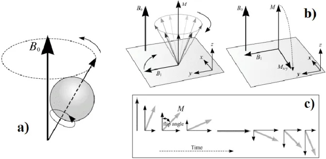
Figure 1. Schematic represents a) precession of magnetic moment around B0, b) effect of RF radiation on net magnetic momentum which is tilted from its original orientation (z-axis) into transverse plane
(x-y), and c) flip angle [12]. ... 9
Figure 2. a) Longitudinal and b) Transverse relaxation time of magnetic moment after termination of RF [13] ... 10
Figure 3. Schematic representation of the inner, second and outer sphere contributions on relaxation time [18] ... 12
Figure 4. Orientation-dependent dipolar field experienced by a neighboring spin ... 14
Figure 5. Schematic of commercial Gd-based clinical approved MRI contrast agents [25] ... 21
Figure 6. Schematic of targeted CAs in tumor cells passively and actively [33] ... 23
Figure 7. Developed macrocyclic chelators for biomedical application [4] ... 24
Figure 8. Structure of Macrocycle chelator as targeting MRI CAs ... 24
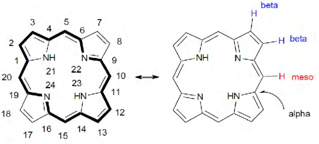
Figure 9. Schematic of porphine and peripheral position of atoms in porphine structure ... 26
Figure 10. The Rothemund synthesis of meso-substituted porphyrin ... 27
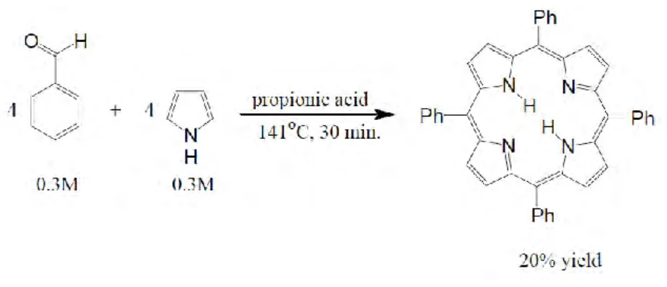
Figure 11. The Aldler-Longo method for preparing meso-substituted porphyrin ... 27
Figure 12. Two steps synthesis of porphyrin at room temperature ... 28
Figure 13. The MacDonald type 2+2 condensation method ... 29
Figure 14. The Gouterman’s four orbital models for D2h symmetry free-base porphyrin (top) and for D4h symmetry metalloporphyrin [56] ... 30
Figure 15. Typical UV-visible spectra of a) free-base and b) metallated porphyrin ... 31
Figure 16. UV-visible absorption spectrum of porphyrin with its typical Soret and Q bands ... 32
Figure 17. Schematically presents the photodynamic therapy using photosensitizers [64] ... 33
Figure 18. T1 weighted images of healthy rats after postinjection of Mn (TPPS3)2 from spin echo sequences at 3T compared with those of after postinjection of conventional CAs Gd-DTPA as reference [87] ... 37
Figure 19. T1 weighted spin echo of rat after pre and postinjection of Mn-porphyrins such as Mn-TCP, Mn(TPPS) and MnP2 (Mn(TPPS3)2) in comparison with Gd-DTPA as a reference at 3T. yellow circle: left kidney, blue circle: bladder [78] ... 38
Figure 20. MRI signal intensity after postinjection of different Gd(III) compounds and their distribution in melanoma xenografts in nude mice after 24h [88] ... 39
Figure 21. Schematic presents diffusing of A) low molecular weight and B) macromolecular CAs from tumor vessels into the interstitial space [93] ... 40
Figure 22. Structure of coupling L-tartaric acid to Gd-DTPA with two degree of polymerization of n=12 (Gd4(H2O)) and n=19 (Gd10(H2O)) ... 42
Figure 23. Structure a)DTPA-HMD and b)DTPA-CHD linear polymers and evaluated the relaxometry properties of two Gd complexes [104] ... 42
Figure 24. Structure and physicochemical parameters of GDCP and GDCEP [105] ... 43
Figure 25. The classification of developed polymeric nanocarries A) dendrimer, B) liposomes, C) polymer-CAs conjugated, D) polymeric nanosphere, E) polymer core-shell nanoparticles [110] ... 44
Figure 26. Fabrication of chitosan from chitin by modulation of deacetylation degree ... 45
Figure 27. In-vivo MR images of mice with T6-17 flank tumors [147] ... 50
Figure 28. T1-weighted of rat liver postinteravenous injection of Gd-DTPA-CS (0.08 mmol/kg Gd) and Gd-DTPA (tail vein) into rat after A) 0 min, B) 5 min, C) 15 min, D) 30 min and E) 90 min [146] ... 51
viii Figure 29. T1-weighted of rat kidney postinteravenous injection of Gd-DTPA-CS (0.08 mmol/kg Gd) and Gd-DTPA (tail vein) into rat after A)0 min, B) 5 min, C) 15 min, D) 30 min and E) 90 min [146]
... 51
Figure 30. a) Different sized CdSe colloids irradiated with UV-visible light and emit different color light b)Emission wavelength of QDs at different particle size[164] ... 52
Figure 31. Algorithm of molecular dynamic simulation ... 59
Figure 32. Schematic explicits simulation box and radial distribution evaluated ... 60
Figure 33.I. Snapshot of particle during simulation: a) 0 ps, b) 13.8 ps, c) 16.3 ps, d) 28.8 ps, e) 41.3 ps, f) 78.9 ps, g) 167 ps, h) 479.5 ps, i) 1100 ps, II. Potential energy of system during MDs time, III. Enlargened snapshot of particle at 479.5 ps, IV. Black balls are atoms with high mobility in the last 1 ps [248] ... 65
Figure 34. 3D snapshot of ZnS 3 nm MDs a) in vacuum, and b) with surface-bound water S atoms yellow, Zn red, O blue, H light blue [244] ... 67
Figure 35. a) ZnS3 and Zn2S3 first cluster formed, b) Zn6S8 cluster after 1.5 ns, c) cluster formation at 500 K, d) Zn9S11 bubble cluster after 6 ns. Yellow stick : S; blue stick : Zn; red sticks : O; and white sticks : H [251]. ... 68
Figure 36. Schematic of Gd(TPyP) synthesis procedure ... 72
Figure 37. Procedure of CNs preparation ... 76
Figure 38. Chemical conjugation of Gd(TPyP)-CNs ... 76
Figure 39. Passive loading of Gd(TPyP)-CNs ... 77
Figure 40. UV-visible absorption spectra of TPyPH2 and Gd(TPyP) dispersed in ethanol at ambient temperature ... 89
Figure 41. FTIR spectra of a) TPyPH2 and b) Gd(TPyP) ... 91
Figure 42. Right: UV-vis spectrum of Fe(TMPyP in water and Left: r1 and r2 of Fe(TMPyP) in water at B0=0.47 T and T=37°C ... 93
Figure 43. Longitudinal and transverse relaxation rates [(1/T1) and (1/T2)] of Mn(TSPP) versus the Mn(III) concentration in water at B0=0.47 T and T=37°C ... 94
Figure 44. Longitudinal and transverse relaxivities r1 and r2 of Gd-DOTA in water and in the mixture of water/ ethanol at B0=0.47 T and T=37°C ... 95
Figure 45. r1 and r2 of Gd(TPyP) in ethanol at B0=0.47 T and T=37°C ... 96
Figure 46. T1 (TR=400 ms, TE=8 ms) and T2 (TR=1500 ms, TE=40 ms) weighted spin echo MR images of different concentration of Mn(TSPP) and Fe (TMePyP) in water at 3T and 25°C... 98
Figure 47. T1 (TR=400 ms and TE=8 ms) and T2 (TR=1500 ms, TE=40 ms) weighted spin echo MR images of different concentration of Gd(TPyP) in ethanol and Gd-Dota in water and Gd-Dota in water/ethanol at 3T and 25°C ... 99
Figure 48. r1 and r2 relaxivities of Mn(TSPP) and Fe(TMPyP) colloids measured via MRI at 3T and 25°C and NMR relaxometry at 0.47T and 37°C ... 100
Figure 49. The r1 and r2 relaxivity of Gd(TPyP) and Gd-DOTA solution at 3T and 25°C and 0.47T and 37°C ... 100
Figure 50. CNs SEM images a) before and b) after sonication. Particle preparation conditions: LMv chitosan concentration = 0.7 mg/mL. TPP concentration=1.25 mg/mL ... 106
Figure 51. FT-IR spectra of bulk chitosan (Mw=60-120 kDa, degree of deacetylation≥93%), and Chitosan nanoparticles ... 107
Figure 52. UV-Vis spectra of Gd(TPyP) in ethanol, NPs-1 and NPs-2: Gd(TPyP)-CNs via chemical conjugation, NPs-3: Gd(TPyP)-CNs via passive method ... 109
Figure 53. UV-visible spectra of Gd(TPyP)-CNs with different concentration of Gd(TPyP) ... 110
ix Figure 55. ICP results versus absorbance of Gd(TPyP)-CNs after conjugation of different quantities of Gd(TPyP) with CNs ... 111 Figure 56. Entrapment efficiency (EE), loading capacity (LC) and yield % for different CNs:
Gd(TPyP) ratios ... 112 Figure 57. SEM image of Gd(TPyP)-CNs with ratio of 3:1 ... 112 Figure 58. DLS results of optimized chitosan nanoparticles and Gd(TPyP)-CNs with ratio of 3:1 ... 113 Figure 59. EDX spectra of Gd(TPyP)-CNs with different ratio of Gd(TPyP):CNs a) sample 1 (0.5:1 mg), b) sample 2 (1:1 mg), c) sample 3 (2:1 mg) and d) sample 4 (3:1 mg) ... 113 Figure 60. FT-IR spectra of a) CNs, b) Gd(TPyP), c)Gd(TPyP)-CNs ... 114 Figure 61. T1 (TR=400 ms, TE=8 ms) and T2 (TR=1500 ms, TE=40 ms) weighted spin echo MR images of different concentration of Gd(TPyP)-CNs in water at 3T and 25°C... 115 Figure 62. Longitudinal and transverse relaxation rates [(1/T1) and (1/T2)] of Gd(TPyP)-CNs versus the Gd(III) concentrations in water at B0=3T and T=25°C ... 116 Figure 63. r1 and r2 relaxivity of Gd(TPyP) encapsulated with chitosan nanoparticles, Gd(TPyP) and Gd-DOTA at 3T and 25°C ... 116 Figure 64. The XRD patterns of the as-prepared MnxZn1-xS (x=0.1, 0.2, and 0.3) ... 118 Figure 65. TEM image of Mn-doped ZnS nanoparticles with different Mn content... 119 Figure 66. Photoluminescence emission spectra of MnxZn1-xS (0.1≤x≤0.3) recorded for λexc=405 nm at room temperature , inset the emission observed from a) Mn0.1Zn0.9S and b)ZnS at 325 wavelength . 120 Figure 67. The schematic diagram of energy-level of Mn doped ZnS nanoparticles corresponding to photoluminescence spectra[348] ... 122 Figure 68. Magnetization versus magnetic field up to 50 kOe for MnxZn1-xS nanoparticles with
different Mn contents (x=0.1, 0.2, and 0.3) at 300K ... 122 Figure 69. Susceptibility versus temperature and in the inset the temperature dependence of inverse magnetic susceptibility of Mn-doped ZnS with different dopant concentrations (0.1≤x≤0.3) at 2kOe ... 123 Figure 70. T1 (3T, TR=400 ms and TE=8 ms) and T2(3T.,TR=1500 ms and TE=40 ms) weighted images of ZnS as reference and MnxZn1-xS (0.1≤x≤0.3) at 3T and 25°C ... 124 Figure 71. Longitudinal and transverse relaxation rates (1/T1) of a) Mn0.1Zn0.9S, b) Mn0.2Zn0.8S and c) Mn0.3Zn0.7S versus the Mn(II) concentrations in aqueous solution at B0=3T and T=25°C ... 125 Figure 72. Schematic of Mn:ZnS capped with mercaptoacetic acid and enlarge carboxylic acid
interaction with water molecules ... 126 Figure 73. Magnetization versus magnetic field up to 50 kOe for Mn0.3Zn0.9S nanoparticles with different particle sizes at 300K ... 128 Figure 74. T1 (TR=400 ms, TE=8 ms) and T2 (TR=1500 ms, TE=50 ms) weighted spin echo MR images of different concentrations of Mn0.3Zn0.7S with different particle size in water at 3T and 25°C ... 129 Figure 75. The longitudinal and transverse relaxation rates (1/T1 and 1/T2) of Mn0.3Zn0.7S with
different particle sizes versus the Mn(II) concentration in water at B0=3 T and T=25°C ... 130 Figure 76. Radial distribution of Zn-Zn and Zn-S and associated coordination numbers ... 132 Figure 77. RDFs and corresponding coordination number of a) Mn-Mn, b) Mn-Zn, c) Mn-S, d) Zn-Zn and e) Zn-S, S-S of MnxZn1-xS (x=0.1, 0.2, 0.3) at 300 K and 1 bar ... 133 Figure 78. Surface [110] crystal structure of a) ZnS and b) MnZnS, yellow : S atom, red : Zn, and grey color : Mn ... 135 Figure 79. Time-dependent of potential energy (eV) of simulated ZnS and MnxZn1-xS (x=0.1, 0.2, 0.3) crystal structure at 300K and 1bar ... 136
x Figure 80. Radial distributions gO-O(r), gO-H(r), and gH-H(r) with corresponding coordination number of water using SPC/E, and TIP3P models ... 137 Figure 81. RDFs and corresponding integration of a) Zn-Zn, Zn-S, b)Zn-O, Zn-H, and c)S-H, S-O 139 Figure 82. Time -dependent of potential energy (eV), Temperature (K), and pressure (kbar) of ZnS in aqueous solution ... 140 Figure 83. RDFs and corresponding coordination number of Mn-O, Mn-H ... 141 Figure 84. RDFs and corresponding CN of Mn-Mn, Mn-S, Mn-Zn, Mn-O, Mn-H, Zn-O, Zn-H, and S-O of MnxZn1-xS (x=0.1, 0.2, 0.3) nanoparticles in aqueous solution ... 144 Figure 85. Snapshot of relaxed system containing water molecules and MnZnS nanoparticles ... 145 Figure 86. Time-dependent of potential energy (eV) of Mn0.1Zn0.9S, Mn0.2Zn0.8S, and Mn0.3Zn0.7S surrounded with water molecules ... 146
xi
List of Tables
Table 1. Available commercial Gd-based MRI contrast agents ... 22
Table 2. List of studied metalloporphyrins and their relaxivities ... 35
Table 3. Methods employed for fabrication of chitosan nanoparticles (CNs) [114] ... 46
Table 4. List of most used potential developed in DL_POLY ... 62
Table 5. Potential parameters developed by Wright and Jackson for model ZnS structure and comparing experimental and calculated structural results [246] ... 64
Table 6. Interatomic potential values used for study incorporation of Cd, Mn, and Fe ions into ZnS sphalerite [249],[250] ... 66
Table 7. Weighted amount and concentration of metalloporphyrins ... 72
Table 8. The potential parameters for simulation of ZnS ... 83
Table 9 . The potential parameters for MnZnS solid structure simulation ... 84
Table 10. Buckingham potential [267] ... 85
Table 11. FT-IR peaks of TPyPH2 and Gd(TPyP) ... 90
Table 12. Longitudinal and transverse relaxation time (T1 and T2) of Mn(TSPP) and Fe(TMPyP) dissolved in distilled water at 20 MHz and 37°C ... 92
Table 13. T1 and T2 relaxation times of Gd-DOTA diluted in water and in the mixture of water/ethanol at 20 MHz and 37°C ... 94
Table 14. Longitudinal (T1) and transverse (T2) relaxation times of Gd(TPyP) at 20 MHz and 37°C 95 Table 15. Mean particle size (nm) and PdI values of CNs in distilled water from different chitosan concentration (mg/mL) with two different deacetylation degree (85% and 93%), TPP=1.25 mg/mL, T=20°C ... 103
Table 16. Effect of stirring rate and time of stirring on average CNs particle size and PdI ... 105
Table 17. The concentration of Gd(TPyP) in water and UV-visible absorbance (a.u.) ... 110
Table 18. Physico-chemical characteristics of MnxZn1-xS such as chemical composition from EDX and XRF analyses, and the average crystal size <LXRD> from XRD and <DTEM> the average particle diameters from statistical analysis of TEM images ... 119
Table 19. Particle size of Mn0.3Zn0.7S evaluated from TEM images and XRD spectrum ... 128
Table 20 . Characteristic sphalerite structure of MnZnS and ZnS from simulation and experiments. 134 Table 21. Comparison of the characteristic properties of various water models and experiment at 298K ... 137
Table 22. RDFs of ZnS interaction with water molecules ... 138
Table 23. The characteristic RDF obtained from MC, MD, QM/MM simulations ... 142
Table 24. RDF and CN of first coordination shell obtained for MnxZn1-xS -H20 (x=0.1, 0.2, 0.3) and ZnS+ H2O ... 143
3
A. General introduction
In medical diagnostics, visualizing molecular processes with cellular resolution is required for early diagnosis and therapeutic approaches. Thereby, considerable efforts have been devoted toward developing various imaging modalities. Each available imaging modality has its own strengths and weaknesses in terms of sensitivity, spatial resolution, target-to-background contrast or potential in clinical applications. After the first visualization of the human body via magnetic resonance imaging (MRI) in 1977 [1], [2] , MRI has become the most widespread clinical diagnostic imaging technique in cancer therapy. MRI offers several significant advantages over other modalities such as high spatial resolution, noninvasiveness, absence of ionizing radiation, and capability to elicit both anatomic and physiologic information simultaneously [3].
However, MRI is emerging an advantageous technique; overriding challenge with MRI is its relatively low sensitively (insufficient contrast) for label detection. In order to better distinguish targeted tissue from surrounding tissue, contrast of the images needs to be enhanced. The contrast of MRI could be affected either by intrinsic (T1, T2 T2*,
proton-density, flow, chemical environment, diffusion and perfusion) or extrinsic (pulse sequence, acquisition parameters (TE and TR, flip angel, etc.), strength of applied field and contrast agents) parameters. One common approach to overcome the lack of MRI sensitivity is applying the contrast agents to provide additional contrast. A tremendous effort has been spent on designing contrast agents which exhibits high relaxivity, low toxicity, specificity, and suitable long intravascular duration and excretion time.
Macrocyclic ligands are widely utilized as the metal chelators owing to high thermodynamic and kinetic stability [4]. Among the studied macrocyclic chelator, porphyrin has attracted much attention in cancer diagnosis and treatment due to its feature preferential uptake by tumor cells (including sarcomas, carcinomas, and atheromatous plaque) [5] while the reasons for this selectivity remain obscure till now. After the first report about high efficiency of water soluble Mn(II)-mesoporphyrin as a tumor targeting MRI contrast agent [6], numerous works have been devoted to study the potential of various water soluble Mn(II) and Fe(II) mesoporphyrins as MRI contrast agents. Nonetheless, low stability of Gd(III)-mesoporphyrins has prevented in development of these complexes. Metallated meso-tetra-pyridyle porphyrin is considered as an axial-ligand stretch due to the coordination of the metal with one nitrogen atom coming from the adjacent porphine molecules which can improve its stability [7]. One way to improve water solubility, is by encapsulating in or covalently attaching the CA on the
4
surface of nanocarriers, leading to improving simultaneously stability, biocompatibility, and the release of paramagnetic ions. Over the last decades, numerous nanocarriers have been explored as platforms for paramagnetic-labeling and/or encapsulation, including polymers, proteins, dendrimers, micelles, and vesicles. Among the studied polymers, chitosan has been receiving much attention in drug delivery and molecular imaging owing to its characteristic properties, including biocompatibility, biodegradability, nontoxicity, and mucoadhesive properties [8], [9]. Hence, conjugation/or encapsulation of metallated- meso-tetra-pyridyle porphyrin with chitosan could be considered as a novel contrast agent.
On the other hand, developing favorable multifunctional imaging probes becomes increasingly more demanding these days in order to obtain complementary physiological and anatomical information and improving the detection of tumor tissues. Nanoparticles offer an ideal platform for developing dual modality probes in molecular imaging techniques owing to their high surface to volume ratio and the possibility to perform surface modification, functionalization and bioconjugation. In this context, quantum dots (QDs) doped with paramagnetic metal ions have been extensively investigated as dual magneto optical cancer probes. Mn-doped QDs are some of the most investigated QDs in medical imaging. Although, research has been mostly focused on the potential of manganese-doped QDs as a fluorescent bio-label [10], its efficiency as an MRI contrast agent is less well studied. Moreover, the majority of Mn-doped QDs as both a MRI contrast agent and a fluorescence label are core/shell structured nanoparticles. While doping of metal ions on the surface of QDs could be a new approach to design the dual agents (i.e. fluorescence and MRI agents) which offers an opportunity to improve the relaxivity of QDs.
Besides the experimental studies, the computational studies allow to gain detailed information about the structure of the paramagnetic substance, solvent, intramolecular interactions of the paramagnetic species in aqueous solution and dynamics of molecules in system [11]. Molecular dynamic simulation (MDs) is one of the most utilized numerical techniques to approximate macroscopic properties of the system. MDs is widely used to understand the dynamic and thermodynamic properties of materials and living matter by observing the position of certain number of atoms/particles over given period. Thus, modeling the contrast agents surrounded with water molecules via molecular dynamic simulation permits us to obtain reliable insight through interaction between a paramagnetic ion and solvation water, while the long-term goal is understanding the relaxation mechanism.
5
B. Objective of thesis
The main aim of my work is developing two new paramagnetic complexes as magnetic resonance imaging longitudinal MRI contrast agents in the form of macromolecular and nanoparticular contrast agents.
1. Developing Gd-meso-tetra-pyridyle porphyrin conjugated with chitosan nanoparticles, which exhibit the high efficiency as MRI contrast agents with a great potential in biomedical applications owing to interesting chitosan properties such as biocompatibility, biodegradability, and mucoadhesive.
2. Developing Mn-doped ZnS quantum dots with high Mn dopant concentrations, in which the majority of Mn lies close to or on the surface of ZnS to extend their application as MRI contrast agents. In order to obtain significant insight about Mn:ZnS interaction with surrounding water molecules, molecular dynamic simulation is carried out for better understanding the relaxation mechanisms of Mn-doped ZnS dispersed in water. Then the simulated results correlate with experimental r1 relaxivity as a function of Mn dopant concentration.
C. Thesis outline
The theory of relaxation mechanism is described in Chapter 2. It provides the necessary basics of MRI and relaxation mechanism of paramagnetic contrast agents. In Chapter 3, the literature related to the objective of thesis is reviewed. Owing to the interdisciplinary character of this work, the literature review chapter is composed of four major parts. The first part provides an overview of metalloprphyrin complexes and their in-vitro and in-vivo efficiency as MRI contrast agents. The second part describes the potential of different developed macromolecular contrast agents. Afterwards, the third part of the literature review deals with the potential of quantum dots as MRI contrast agents. Finally, the numerical simulation background of nanoparticles in particular those used for evaluating/interpreting the dynamic of QDs in aqueous solution will be explained. Chapter 4 concerns methodological and characterization of both developed paramagnetic complexes. Meantime, molecular dynamic simulations procedure and the potential parameters are explained. Chapter 5 deals with the results and discussion of physicochemical characterization of two novel developed contrast agents and their efficiency as MRI contrast enhancers. The simulated results of Mn:ZnS QDs
6
in vacuum and in aqueous media (water) are then described in the last section of Chapter 5. Finally in the Chapter 6, the contributions of my thesis work is summarized by providing some helpful prospectives to future research directions.
9
A. Basic principle of MRI
Magnetic Resonance Imaging (MRI) is based on the magnetic properties of water protons (hydrogen) and on the water protons interaction with both applied magnetic field and radiofrequency producing highly detailed images of the human body. The hydrogen atom has a net magnetic moment. Therefore, in the absence of an external magnetic field, protons are randomly orientated. The protons tend to align with or against the magnetic field and precess around it. The frequency of precession is described by Larmor’s equation
Ω=γB (1)
where ω is the frequency precession and γ is the gyromagnetic ratio, which is a constant, and B is strength of applied field. During application of an external magnetic field (B0), the
majority of protons align along the field direction into the low energy state, giving rise to a net magnetization in the direction of B0. The second weaker magnetic field, radiofrequency
(RF) pulse, is applied in a perpendicular direction to the first field and oscillated at a Larmor
frequency. This causes the magnetic moment (M) to tilt away from B0 and flip about an angle
dependent on the pulse duration and amplitude as presented in Fig. 1. After the termination of
the RF pulse, the magnetization will not precess perpetually around the B0-field but will return
to its equilibrium position along the z-axis (direction of B0).
Figure 1. Schematic represents a) precession of magnetic moment around B0, b) effect of RF
radiation on net magnetic momentum which is tilted from its original orientation (z-axis) into transverse plane (x-y), and c) flip angle [12].
10
During relaxation, the nuclei lose energy by emitting their own RF signal. This signal is referred to free-induction decay (FID) response signal, which could be observed thanks to the induced current in a detector coil. After a 90° RF pulse, the amplitude of the signal detected by the coil does not rapidly drop down to zero. The loss of transverse magnetization with time because of spin dephasing is referred to as Free Induction Decay (FID). The Larmor frequencies of distinctive nuclei and their respective contributions are obtained by Fourier transform of this signal.
B. Relaxation time
The return of magnetic moment to its equilibrium state is expressed as relaxation. T1 relaxation (also known as spin-lattice or longitudinal relaxation) is the realignment of spins (M) with the external magnetic field B0 (z-axis). T2 relaxation (also known as T2 decay,
transverse relaxation or spin-spin relaxation) is the decrease of the Mxy component.
Figure 2. a) Longitudinal and b) Transverse relaxation time of magnetic moment after termination of RF [13]
B.1. Longitudinal relaxation time
After the RF pulse, nuclei will dissipate their excess energy as heat and revert to their
Boltzman equilibrium position. Realignment of the nuclei along z-axis (B0), through a process
known as recovery, leads to a gradual increase in the longitudinal magnetization. The time taken for a nucleus to relax back to its equilibrium state is called longitudinal relaxation time. The process of equilibrium restoration is described as follows
11 ) 1 ).( 0 ( ) ( T1 t z z t M e M (2)
where T1 is the time taken for the longitudinal magnetization to be restored.
B.2. Transverse relaxation time
After applying a RF pulse, all the individual spins magnetic moments precess coherently around the z-axis, creating a magnetization component in the xy-plane. The magnetic moments interact with each other causing a decrease in transverse magnetization. The transverse relaxation time corresponds to the time taken for disappearance of magnetization in the xy-plane. The transverse relaxation time is described by the following equation
2 ). 0 ( ) ( T t xy xy t M e M (3)
while T2 is the time taken that the transverse magntizations decay to 37% of its initial value. The relaxation time of water could be shortened by nearby paramagnetic or superparamagnetic particles due to their large electronic magnetic moments (dipoles) in the presence of external magnetic field. Gd (III) with seven and Mn (II) and Fe (II) with five unpaired electrons are the most widely used paramagnetic ions for increasing proton relaxation rate of water molecules.
The efficiency of paramagnetic ions to affect the relaxation times of water protons is evaluated by relaxivity (r1 or r2) which are defined as the increase of relaxation rate (1/T1 or
1/T2) produced by 1mmol per liter of paramagnetic substance (expressed mmol-1.s-1). The r1
and r2 relaxivities are the main physicochemical parameters in development and design of contrast agents. C r T Ti(obs) i(dia) i 1 1 i=1,2 (4) where ) ( 1 obs i
T corresponds the relaxation rate of aqueous system (s
-1 ) , ) ( 1 dia i T relaxation rate of
the solvent (s-1), C concentration of paramagnetic ion (mmol-1) and ri the relaxivity (mmol-1.s -1
12
C. Paramagnetic relaxation time
A quantitative theoretical model has been developed to demonstrate the relaxivity of contrast agents [14]. The paramagnetic relaxation of water protons originates from the dipole-dipole interactions between proton nuclear spins of water molecules and the fluctuating local magnetic field, which is produced from unpaired electron spins of the paramagnetic ions [15]. The paramagnetic relaxation is explained by inner, second, and outer sphere contributions [16], as shown in Fig. 3. The inner sphere contribution arises from interaction of water molecule(s) in the first coordination sphere with paramagnetic ions which transmitted to bulk via chemical exchange [17]. Besides the inner sphere coordinated water, there are some water molecules that may be bonded to the ligand (hydrogen-bonded) or to the inner sphere water molecule(s). These water molecules also contribute to overall paramagnetic relaxation, identifying as second sphere contribution [17]. The bulk water molecules, which have diffused around the paramagnetic center, also experience the paramagnetic effect. This relaxation mechanism is defined as outer sphere contribution. Thereby, total paramagnetic relaxation rate can be expressed as follows
2 , 1 1 1 1 1 i T T T T OS ip SS ip IS ip ip (5)
where IS, SS and OS stand from inner, second and outer sphere, respectively.
Figure 3. Schematic representation of the inner, second and outer sphere contributions on relaxation time [18]
13
C.1. Inner Sphere Proton relaxivity
The relaxivity of bulk water is based on exchange of coordinated water with paramagnetic ions, defined as
m m p T O H q R 1 2 1 (6)
H O
q T T T R m m m m m m m m P 2 2 2 1 1 2 2 1 1 2 1 2 ) ( ) ( 1 (7) Where m T1 1 and m T2 1are longitudinal and transverse relaxivities, mis the chemical shift
difference between coordinated water and bulk water, m is lifetime of coordinated water in
first sphere, and q is the number of coordinated water moolecules. The relaxation of a coordinated water proton is governed by dipole-dipole coupling (dd) between the paramagnetic ion and hydrogen of water [19], scalar relaxation (sc) [19], and curie spin (cs) relaxations [20]. It is noteworthy that at high magnetic field of 1.5T and higher, only dipolar relaxation contributes to longitudinal relaxation rate while all three mechanisms can contribute to transverse relaxation rate.
2 1 2 1 2 2 2 2 6 2 2 2 2 0 1 1 3 1 7 ) 1 ( 4 15 2 1 c H c c S c MH B e H DD r S S g T (8) 2 2 2 1 3 1 )) 1 ( ( 2 1 SC S SC SC A S S T (9) 2 2 2 2 6 2 2 2 4 4 2 2 0 1 1 3 ) 3 ( ) 1 ( 2 4 1 H MH B B e H CS r T K S S g T (10)
Moreover, transverse relaxivity arises from inner sphere contribution is defined as follows
2 1 2 1 2 2 2 2 6 2 2 2 2 0 2 1 3 1 13 4 ) 1 ( 4 15 1 1 c H c c S c c MH B e H DD r S S g T (11)
2 2 2 2 1 ) 1 ( 3 1 1 SC S SC SC S S A T (12)14 2 2 2 2 6 2 2 2 4 4 2 2 0 2 1 4 ) 3 ( ) 1 ( 4 5 1 1 H MH B B e H CS r T K S S g T (13)
Where γ is the nuclear gyromagnetic ratio, g electron factor, μB Bohr magneton, rMH the
electron spin-proton distance, τc correlation time, and ωI and ωH are the nuclear and electron
Larmor frequencies, respectively. The correlation time (τc) is defined as
ie R m ci T 1 1 1 1 i=1,2 (14)
while τR is the rotational correlation time and T1e and T2e are longitudinal and transverse
electron spin relaxation time.
C.1.1. Dipolar interaction
The interaction between two magnetic moments causes the field fluctuation. The alignment of spin to magnetic field influence the local dipolar field of neighboring spin (as shown in Fig. 4). This interaction is known as dipole-dipole or dipolar coupling. The interaction could be heteronuclear or homonuclear, between different nuclei or the same sort, respectively. The dipolar interaction plays a main role in the relaxation mechanism, especially for the higher spin system.
15 C.1.2. Scalar interaction
The scalar interaction occurs when the nucleus-electron distance is about the nucleus radius. Thereby, the nuclei bound directly to the paramagnetic specie undergoing the scalar interaction. The scalar interaction is mainly influenced by electron spin relaxation and by water exchange rates and remains unaffected by orientation of the molecule. The correlation time of scalar interaction is given by
M ie SCi T 1 1 1 i=1,2 (15) For the CAs composed of paramagnetic ions with S>1/2, electron spin relaxations are interpreted in terms of Zero Field Splitting (ZFS) interaction. The electronic relaxation is field dependent. For Gd(III) complex the rates are interpreted as follows
4 ( 1) 3
( , ) 4 (2 , )
50 2 1 2 1 v S v S v e J J S S T (16)
4 ( 1) 3
3 (0, ) 5 ( , ) 2 (2 , )
50 1 1 2 2 v S v S v v e J J J S S T (17)
0 2 3 ) 1 ( 4 5 S v S S (18)Where τv is correlation time for modulation of ZFS interaction, Δ amplitude of transient ZFS
and τS0 electron spin relaxation time at zero field.
C.1.3. Curie relaxation
In paramagnetic system, due to the Boltzman distribution there is a difference in the populations of electron spin energy levels, which induce a magnetic moment. This perturbation can influence the relaxation mechanism which is known as curie relaxation.
Referring equations 6 to 18, numerous parameters have an impact on protons relaxivity from inner sphere contributions.
1. Rotational coordination time (R): reorientation of vector between paramagnetic ion and the water molecule proton.
16
2. Electronic relaxation time (T1e,T2e): the process of returning to equilibrium state of magnetization associated to electrons during transitions between electronic levels of paramagnetic center.
3. Number of coordinated water molecules (q)
4. Distance between proton and paramagnetic ions (rMH) have sixth-power dependence
and influence significantly the dipolar relaxation rate.
5. Residence time of coordinated water (M): exchange between water molecules
surrounding the complex and water coordinated to the metal ion. The residency time should be long enough to increase the probability of relaxation to occur meanwhile short enough to exchange the relaxed water molecule with the bulk water [21].
C.2. Second sphere relaxivity
The second sphere relaxation pathway in principle depends on the same parameters as the inner sphere term. The contribution is enhanced by slowing down rotational correlation time, increasing the number of hydrogen-bonded waters and their residency lifetime. The distinguishing contribution of the second sphere from the outer sphere term is very difficult.
The effect of second sphere term on relaxivity has been reported for [Gd-DOTP]5- (q=0) with
human serum albumin (HAS). The relaxivity enhancement of [Gd-DOTP]5- in the presence of
(HAS) has been attributed to the presence of exchangeable protons on proteins close to the interaction site of the complex and from hydrogen-bonded water molecules in the second sphere shell.
C.3. Outer sphere relaxivity
Outer sphere theory demonstrates the relaxation induced by diffusion of water molecules within the magnetic field gradient around the paramagnetic hydrated ion [22]. This mechanism may contribute to the relaxivity of paramagnetic complexes at the imaging fields, arising from modulation of dipolar interaction of the paramagnetic ions with water molecules which are diffusing next to the surface of the complex. The component relaxivity arising from the outer sphere has been estimated by a expression derived by Freed [23].
)7 ( ) 3 ( )
( 2 S 1 H OS OS ip J J aD CA C r (19)17 2 / 3 2 / 1 2 / 1 ) ( 9 / 1 ) ( 9 / 4 ) ( 1 ) ( 4 1 1 Re ) ( je d d je d d je d d je d d T i T i T i T i J j=1,2 (20)
Where a is the distance of closest approach, D diffusion constant, and τD translational
correlation time equal to a2/D, constant COS (5.8x10⁻¹⁰ m6mol-1s-2) and J(ω) is the non-Lorentzian spectral density. At the imaging field, the outer sphere relaxivity depends on distance of closest approach, which attributes to the molecular dimension and charge distribution of complex, and on the relative diffusion coefficient of solute and solvent.
21
Over decades, much effort has been focused on developing the MRI contrast agents with high efficiency. However, until now only some of these agents are clinically approved. The Gd-based contrast agents available for clinical use, presented in Fig. 5 and summarized in Table 1, are nine coordinated complexes, binding with eight ligand sites and one water molecule,
with molecular weight less than 1000 Da. Among the listed CAs, [Gd(DTPA)(H2O)], first
approved contrast agent [24], [Gd(DOTA)(H2O)], [Gd(BOPTA)(H2O)] and MS-325 are ionic
CAs while the rest are neutral CAs.
Figure 5. Schematic of commercial Gd-based clinical approved MRI contrast agents [25]
The first generation of currently available clinical contrast agents is non-specific extracellular MRI CAs. They distribute into the intravascular and interstitial space. This allows us to evaluate the physiological parameters, including renal function and status or existence of blood brain barriers [26]. Non-specificity of conventional CAs causes their poor performance for early diagnosis and imaging of specific organs. However, CAs with preferential uptake to
22
a particular tissue would improve the diagnostic accuracy. This type of CAs has been named as targeted CAs or second generation CAs.
Table 1. Available commercial Gd-based MRI contrast agents
Chemical name Generic name Brand name
Charge Company Relaxivity (mM-1s-1) (Gd(DTPA)(H20)] Gadopentetate dimeglumine Magnevist 2- Schering(Germany) +r1=4.9, r2=6.3 [Gd(DOTA)(H20)] Gadoterate meglumine
Dotarem 1- Guerbet (France) r1=3.4, r2=4.8, B0=1.0T [Gd(DTPA-BMA)(H20)] Gadodiamide Omniscan 0 Amersham *r1=5.4
[Gd(HP-D03A)(H20)] Gadoteridol ProHance 0 Bracco (Italy) *r1=5.4
[Gd(D03A-butrol)(H20)] Gadobutrol Gadovist 0 Schering(Germany) r1=3.6, B0=1.0
T
(Gd(DTPA-BMEA)(H20)]
Gadoversetamide OptiMARK 0 Mallinckrodt (U. S.)
♦[Gd(BOPTA)(H2O)] Gadobenate
Dimeglumine
MultiHance 2- Bracco spa (Italy) +r1 = 9.7, r2 =
12.5
♦Gd-EOB-DTPA Gadoxetic acid Primovist 2- Schering (Germany) *r
1 = 6.9, r2 = 8.7 MS-325 Gadofosveset trisodium Vasovist 3- EPIX/Schering, Malinckrodt r1=27.7, r2=72.6, 1.5T
+ In heparinized human plasma, at 39°C * In citrated human plasma, at 37°C
♦ Second generation of CAs
Gd[BOPTA] and Gd-EOB-DTPA are classified as second generation contrast agents. Second generation CAs exhibit responsive behavior to physiochemical environments such as pH of solution, temperature, redox potential, metal ion concentration (Zn, Ca, Cu), and enzyme activity. These agents have shown the selectively uptake by a particular kind of cell. For
instant, [Gd (BOPTA)]2- has shown great efficiency in the imaging of liver and myocardium
[27]. Moreover, it has been used in applications of perfusion cardiac MRI for the diagnosis of coronary artery disease, cardiac tumors, inflammations and different types of
cardiomyopathies [27]. [Gd(EOB-DTPA)]2- is applied for detection of liver metastases [28].
Nowadays, much research has been focused on designing targeted CA.
A. Tumor-Targeting contrast agents
In actively growing tumor cells with volume greater than 2 mm3, delivery of nutrients and oxygen become limited. In order to supply oxygen and nutrients to tumor cells, new blood vessels form around tumor cells with enlarge gap junction of 100 nm to 2μm [29]. These new vessels are irregular and poorly organized which shows leaky fenestrations. This leads the extravasations of small macromolecules and nanoparticles smaller than 100 nm, which are out
23
of vasculature, into tumor cells [30]. Moreover, tumor cells show higher compound retention time compared with healthy tissues because of their inefficient lymphatic drainage [31], [32]. These two features provide an enhanced permeability and retention (EPR) effect in tumor cells that is playing an important role for passive targeting and accumulation of contrast agents in tumor interstitium [29]. The accumulation of targeting agents in tumor cells passively or actively is schematically presented in Fig. 6.
Figure 6. Schematic of targeted CAs in tumor cells passively and actively [33]
Furthermore, one method to increase the accumulation of CAs in tumor tissues is surface conjugation of CAs with appropriate ligands to targeting either cell surface or receptor targeting. These CAs have the ability to recognize cellular membrane of specific molecular sites. Thus, by administration of targeting CAs, the concentration of CAs in targeted tissue is much greater than in non-targeted tissue, which enhances the selective tissue’s relaxation and may increase contrast between specific tissue and its surrounding. Whilst some complexes such as porphyrins have shown the intrinsic uptake by tumor cells [34], [35].
A.1. Macrocyclic chelator
Among the available commercial CAs, non-macrocyclic chelators such as DTPA shows a releasing Gd(III) which causes nephrogenic systemic fibrosis disease [4]. Thus, complexes with high stability to chelate the paramagnetic ions are desirable. The advantages of using macrocyclic complexes as chelators is their high thermodynamic, kinetic stability, and ability
24
to tune their coordination environment [4]. In Fig. 7, the most common macrocyclic chelators
used as imaging agents are presented.
Figure 7. Developed macrocyclic chelators for biomedical application [4]
On the other hand, the developed macrocyclic ligands have been modified to target specific tissue or cellular receptors in order to enhance the contrast of MR imaging. For instance, conjugation of macrocycle Gd-Dota to polyarginie oligomers and stilbene derivatives could help Gd-Dota become a targeting MRI CA [36]. Meade and his colleagues succeeded in attaching progesterone derivatives to Gd-DO3A which could be applied as breast cancer prognostic marker, presented in Fig. 8a [37]. In other research, Gd-DO3A have been functionalized with an alkyl group as MRI targeting contrast agents, shown in Fig. 8b [38]. Gd(III) cyclen macrocycle has also been modified for using as bone imaging and therapy by addition of phosphate group in the macrocycle [39].
25
As described before, macrocyclic complexes have been chemically modified to be used as targeting agents. Furthermore, porphyrin is a macrocyclic chelator which has a natural tendency to penetrate into tumor cells.
A.1.1. General reviews of Porphyrins
Porphyrin stems from the Greek word porphura due to its intense purple color. The utility of naturally occurring porphyrin compounds is aa strong incentive for widespread attention in porphyrin chemistry. Porphyrin plays an important role in the metabolism of living organisms. For instance in mammalian blood, hemoglobin is iron substituted porphyrin derivatives. Cytochrome is hemeproteins, which transfer electron to cell respiration.
Adenosylcobalamin or vitamin B12 is another naturally occurring porphyrin, which is made of
cobalt/corrin complex. Corrin is similar to the porphyrin ring while it contains one less methine bridge causing loss of planarity and aromaticity within the macrocycle. While this complex in the body helps in methylation of DNA and producing hemoglobin. Chlorophyll, which is responsible for transfer of photonic energy to the reaction center in plants and plays an important role in photosynthesis, is the other example of a naturally occurring porphyrin derivative.
The simple structural feature of porphyrin (porphine) consists of four pyrrolic units connected through one-carbon methine bridges. The bridging of pyrrole units results in a large and planar macrocyclic structure with unsaturated atomic center. The porphyrin compounds follow Huckel’s rule [40], which estimates the aromatic properties of planar rings. Due to this rule, the number of π electrons in a cyclic ring equals to (4n+2) while n is zero or a positive integer. In porphyrin, n equals to 4 thereby there are 18 π conjugated electrons. It is noteworthy that there are 22 π electrons in porphyrin while just 18 π electrons are delocalized [40]. High stability and astonishing photophysical properties of porphyrin complexes arise from this strong conjugation. The porphyrin can be substituted in different positions. Positions 5,10,15,20 are four meso-substituted positions while 2, 3, 7,8,12,13,17,18 are the eight β-substituted positions, as shown in Fig. 9. The rest are the eight possible α-β-substituted positions. β- and meso positions can be substituted by functional groups. Among the various porphyrin derivatives, meso-substituted porphyrins have received great attention in many fields including solar cell, biomedical, chemical sensor and photodynamic therapy.
26
Figure 9. Schematic of porphine and peripheral position of atoms in porphine structure
As presented in Fig. 9, two pyrrolenine nitrogen atoms in porphyrin rings are capable of accepting protons while two NH groups are capable of losing protons. The losing proton results in the formation of dianion species which makes it suitable to insert metal ions in the core of porphyrin. Free base porphyrin can bind with almost all metals and some semi-metals to form metalloporphyrin complexes. Referring to the position of metal ions in metalloporphyrin, they can be categorized as in plane, out-of-plane or in bimetallic complexes.
A.1.2. Synthesis of meso-substituted porphyrin complex
The arrangement of diverse substituents in specific patterns is the main theme in the synthesis of porphyrins [41]. Control over this arrangement enables us to design and tailor different types of porphyrins for specific applications [41]. Meso-tetraphenylporphyrin has been successfully synthesized for the first time by Rothemund in 1936 [42]. Rothmund has reported the formation of meso-substituted porphyrin in one step using pyrrole and benzaldehyde under acidic conditions in a sealed flask at 150°C for 24h [43] (Fig. 10). The low yield, irreproducible and harsh experimental conditions are the limitation of this set up [44], [45].
27
Figure 10. The Rothemund synthesis of meso-substituted porphyrin
In Rothemund synthesis, the character of substituent on the phenyl ring affects the yields of tetraphenylporphyrin [46]. The reaction and yields of tetrraphenylporphyrin can be accelerated by electron-accepter substituents while electron donor substituents can retard the reaction and reduce the yields [47]. This retardation is attributed to preferable polymerization of pyrrole to obtain polypyrrole.
In 1967, Alder, Longo and coworkers reexamined and modified the Rhotemund method [48]. They reacted benzaldehyde and pyrrole by condensation in refluxing propionic acid in glassware open to the atmosphere [48] (Fig. 11) under 141°C for 30 minutes. Performing the reaction on the large scale is the advantage of Alder’s method. Moreover, this method is much milder than Rothemund’s synthesis conditions and it is compatible with a variety of aldehydes with yields of 20%.
Figure 11. The Aldler-Longo method for preparing meso-substituted porphyrin
However, while the Alder method works better than Rothemund method, it has a limitation such as failing reaction with benzaldehydes, no crystallization of porphyrin , purification problem, and low and often irreproducible yields [49].
28
The Alder method was optimized by Lindsey and coworkers in 1987[50], [51]. In this method, a new strategy for the synthesis of meso-substituted porphyrin has been used. The reaction has been performed using acid-catalyzed pyrrole-aldehyde condensation in the presence of CHCl3 for one hour at room temperature. The first step has been monitored to
obtain maximum porphyrinogen which can be oxidized rapidly to porphyrin with addition of 3 equivalents of quinon oxidant in the 2nd step [52], as shown in Fig. 12. The reaction was carried out under gentle conditions to achieve equilibrium during condensation and to avoid any side reaction. The oxidation of porphyrinogen in the Lindsey method has been carried out by adding p-chloranil, 2,3-dichlor-5,6dicyano-1,4-benzoquinone (DDQ) which require one hour for a complete reaction. This method also has its own limitation such as expensive cost, destroying some porphyrinogen during adding DDQ, requiring large volume of solvent (pyrrole and aldehyde), and difficult purification of porphyrin [53].
Figure 12. Two steps synthesis of porphyrin at room temperature
In the MacDonald method, different meso-substituted trans-porphyrins can be prepared by condensation of a 5-disubstituted dipyrromethane with aldehyde as shown in Fig. 13 [54] . The drawback of this method can be referred to modest yields of porphyrin (10-30%), and condensation in dilute solutions (10 mM). Sometimes the dipyrromethane-aldehyde condensation is not desirable to produce trans-A2B2-porphyrin because of obtaining the
29
Figure 13. The MacDonald type 2+2 condensation method
A.1.3. Electronic absorption Spectrum of porphyrin
For the first time in 1960, the absorption spectrum of porphyrin was successfully explained in terms of four orbital models. Due to four orbital models of Martin Gouterman [55], absorption bands in porphyrin complex originate from transition between two highest occupied molecular orbital (HOMO and HOMO-1 , π orbitals) and two lowest unoccupied molecular orbital’s (LUMO and LUMO+1, π* orbitals) as presented in Fig. 15. For metalloporphyrin
with 4-fold symmetry, the LUMOs are degenerate (labeled as egx and egy) whereas HOMOs
are nearly degenerate (labeled as a1u and a2u). Excited states comes from the transition
between a1u,2u→egx,gy (x-polarization) and those between a1u,2u→egy,gx (y-polarization). These
polarized excited states are mixed and split into two states in energy, lower energy (labeled as Qx and Qy) and higher energy (labeled as Bx and By) states. Lower energy (with less oscillator
strength) and higher energy (with greater oscillator strength) give rise to a Q band and Soret band, respectively. In the case of free base porphyrin, 2- fold symmetry results in nondegeneracy of LUMOs and splitting of Qx and Qy as well as Bx and By transition.
30
Figure 14. The Gouterman’s four orbital models for D2h symmetry free-base porphyrin (top)
and for D4h symmetry metalloporphyrin [56]
As explained, the electronic absorption spectrum of porphyrin contains two distinct regions. The first region, which involves the transition from ground state to the second excited state, is called the Soret band. The Soret band of porphyrin is in the range of 380-500 nm depending on the type of porphyrin- whether meso- or β-substituted. The second region, in the range of 500-700 nm, is called Q band, which involves the weak transition from ground state to the first excited state. Protonation of two inner nitrogen atoms during metallation of porphyrin causes strong changes to the visible absorption spectrum. This change is attributed to more symmetry in protonated (metallated porphyrin) than the free base one that simplifies the Q band pattern.
Based on relative intensities of four Q bands, four basic spectra have been identified in UV-visible spectra of porphyrin, presented in Fig. 14. If the relative intensities of Q bands are in the order of IV>III>II>I, the spectrum is called etio type. This type of spectrum can be observed in β-substitued porphyrin while six or more positions are substituted with groups such as alkyl without any π-electrons. Rhodo type of spectrum could be observed while β-positions of porphyrin have been substituted with groups such as carbonyl or vinyl groups which has π-electrons. This causes a change in the relative intensity of Q bands (III>IV>II>I) and shifting the spectrum to the longer wavelength (redshift). Substituting of two electron-withdrawing groups on opposite pyrrole rings causes a change in maxima absorption
![Figure 2. a) Longitudinal and b) Transverse relaxation time of magnetic moment after termination of RF [13]](https://thumb-eu.123doks.com/thumbv2/123doknet/2242610.17377/28.892.128.789.571.805/figure-longitudinal-transverse-relaxation-magnetic-moment-after-termination.webp)
![Figure 3. Schematic representation of the inner, second and outer sphere contributions on relaxation time [18]](https://thumb-eu.123doks.com/thumbv2/123doknet/2242610.17377/30.892.235.663.756.1083/figure-schematic-representation-inner-second-sphere-contributions-relaxation.webp)
![Figure 5. Schematic of commercial Gd-based clinical approved MRI contrast agents [25]](https://thumb-eu.123doks.com/thumbv2/123doknet/2242610.17377/39.892.110.751.322.886/figure-schematic-commercial-based-clinical-approved-contrast-agents.webp)


![Figure 21. Schematic presents diffusing of A) low molecular weight and B) macromolecular CAs from tumor vessels into the interstitial space [93]](https://thumb-eu.123doks.com/thumbv2/123doknet/2242610.17377/58.892.241.611.92.386/figure-schematic-presents-diffusing-molecular-macromolecular-vessels-interstitial.webp)
![Figure 23. Structure a)DTPA-HMD and b)DTPA-CHD linear polymers and evaluated the relaxometry properties of two Gd complexes [104]](https://thumb-eu.123doks.com/thumbv2/123doknet/2242610.17377/60.892.122.761.828.1054/figure-structure-linear-polymers-evaluated-relaxometry-properties-complexes.webp)