Études probabilistes en théorie des nombres et combinatoire des mots : exemples d’analyse dynamique

(1)

HAL Id: tel-02463068

https://tel.archives-ouvertes.fr/tel-02463068

Submitted on 31 Jan 2020

HAL is a multi-disciplinary open access

archive for the deposit and dissemination of sci-entific research documents, whether they are pub-lished or not. The documents may come from teaching and research institutions in France or abroad, or from public or private research centers.

L’archive ouverte pluridisciplinaire HAL, est destinée au dépôt et à la diffusion de documents scientifiques de niveau recherche, publiés ou non, émanant des établissements d’enseignement et de recherche français ou étrangers, des laboratoires publics ou privés.

Études probabilistes en théorie des nombres et

combinatoire des mots : exemples d’analyse dynamique

Pablo Rotondo

To cite this version:

Pablo Rotondo. Études probabilistes en théorie des nombres et combinatoire des mots : exemples d’analyse dynamique. Number Theory [math.NT]. Université Sorbonne Paris Cité; Universidad de la República (Montevideo), 2018. English. �NNT : 2018USPCC213�. �tel-02463068�

(2)

univ ersit ´e

P

AR

I

S .

D

I

DER

O

T

PARIS 7 THESE DE DOCTORAT DE` UNIVERSIDAD DE LAREPUBLICA ET DE´

L’UNIVERSITE´ SORBONNEPARISCITE´

PREPAR´ EE´ A L` ’UNIVERSITE´ PARISDIDEROT

´

ECOLE DOCTORALE DESCIENCES MATHEMATIQUES DE´

PARISCENTRE ED 386

INSTITUT DERECHERCHE ENINFORMATIQUEFONDAMENTALE

Probabilistic studies in Number Theory and Word

Combinatorics: instances of dynamical analysis

Par Pablo Rotondo

Th`ese de doctorat d’Informatique

Codirigée par Valérie Berthé, Brigitte Vallée et Alfredo Viola

Présentée et soutenue publiquement à l’Université Paris Diderot le 27 septembre 2018 Président du jury Cyril NICAUD Université Paris-Est

Rapporteurs Bruno SALVY INRIA

Pierre ARNOUX Institut de Math´ematique de Luminy Examinateurs Franco ROBLEDO Universidad de la Rep´ublica

Thomas STOLL Université de Lorraine Brigitte VALL ÉE CNRS, Université de Caen Directeurs de thèse Valérie BERTH É CNRS, Université Paris Diderot

(3)

2

Abstract. Dynamical Analysis incorporates tools from dynamical systems, namely the Transfer Operator, into the framework of Analytic Combinatorics, permitting the analysis of numerous algorithms and objects naturally associated with an underlying dynamical system. This dissertation presents, in the integrated framework of Dynamical Analysis, the probabilistic analysis of seemingly distinct problems in a unified way: the probabilistic study of the recurrence function of Sturmian words, and the probabilistic study of the Continued Logarithm algorithm.

Sturmian words are a fundamental family of words in Word Combinatorics. They are in a precise sense the simplest infinite words that are not eventually periodic. Sturmian words have been well studied over the years, notably by Morse and Hedlund (1940) who demonstrated that they present a notable number theoret-ical characterization as discrete codings of lines with irrational slope, relating them naturally to dynamtheoret-ical systems, in particular the Euclidean dynamical system. These words have never been studied from a prob-abilistic perspective. Here, we quantify the recurrence properties of a “random” Sturmian word, which are dictated by the so-called “recurrence function”; we perform a complete asymptotic probabilistic study of this function, quantifying its mean and describing its distribution under two different probabilistic models, which present different virtues: one is a naturally choice from an algorithmic point of view (but is innovative from the point of view of dynamical analysis), while the other allows a natural quantification of the worst-case growth of the recurrence function. We discuss the relation between these two distinct models and their respective techniques, explaining also how the two seemingly different techniques employed could be linked through the use of the Mellin transform. In this dissertation we also discuss our ongoing work regarding two special families of Sturmian words: those associated with a quadratic irrational slope, and those with a rational slope (not properly Sturmian). Our work seems to show the possibility of a unified study.

The Continued Logarithm Algorithm, introduced by Gosper in Hakmem (1978) as a mutation of classical continued fractions, computes the greatest common divisor of two natural numbers by performing division-like steps involving only binary shifts and subtractions. Its worst-case performance was studied recently by Shallit (2016), who showed a precise upper-bound for the number of steps and gave a family of inputs attaining this bound. In this dissertation we employ dynamical analysis to study the average running time of the algorithm, giving precise mathematical constants for the asymptotics, as well as other parameters of interest. The underlying dynamical system is akin to the Euclidean one, and was first studied by Chan (around 2005) from an ergodic point of view, but the presence of powers of 2 in the quotients ingrains into the central parameters a dyadic flavour that cannot be grasped solely by studying this system. We thus introduce a dyadic component and deal with a two-component system. With this new mixed system at hand, we then provide a complete average-case analysis of the algorithm by Dynamical Analysis.

Key words. Dynamical Analysis, dynamical systems, Word Combinatorics, Sturmian words, recurrence functions, greatest common divisor, continued fractions, continued logarithm expansion, transfer operator, Riemann sums, Dirichlet series, Tauberian theorem.

(4)

3

Résumé. L’analyse dynamique intègre des outils propres aux systèmes dynamiques (comme l’opérateur de transfert) au cadre de la combinatoire analytique, et permet ainsi l’analyse d’un grand nombre d’algorithmes et objets qu’on peut associer naturellement à un système dynamique. Dans ce manuscrit de thèse, nous présentons, dans la perspective de l’analyse dynamique, l’étude probabiliste de plusieurs problèmes qui semblent à priori bien différents : l’analyse probabiliste de la fonction de récurrence des mots de Sturm, et l’étude probabiliste de l’algorithme du “logarithme continu”.

Les mots de Sturm constituent une famille omniprésente en combinatoire des mots. Ce sont, dans un sens précis, les mots les plus simples qui ne sont pas ultimement périodiques. Les mots de Sturm ont déjà été beaucoup étudiés, notamment par Morse et Hedlund (1940) qui en ont exhibé une caractérisation fonda-mentale comme des codages discrets de droites à pente irrationnelle. Ce résultat relie ainsi les mots de Sturm au système dynamique d’Euclide. Les mots de Sturm n’avaient jamais été étudiés d’un point de vue probabiliste. Ici nous introduisons deux modèles probabilistes naturels (et bien complémentaires) et y analysons le comportement probabiliste (et asymptotique) de la “fonction de récurrence” ; nous quantifions sa valeur moyenne et décrivons sa distribution sous chacun de ces deux modèles : l’un est naturel du point de vue algorithmique (mais original du point de vue de l’analyse dynamique), et l’autre permet naturellement de quantifier des classes de plus mauvais cas. Nous discutons la relation entre ces deux modèles et leurs méthodes respectives, en exhibant un lien potentiel qui utilise la transformée de Mellin. Nous avons aussi considéré (et c’est un travail en cours qui vise à unifier les approches) les mots associés à deux familles particulières de pentes : les pentes irrationnelles quadratiques, et les pentes rationnelles (qui donnent lieu aux mots de Christoffel).

L’algorithme du logarithme continu est introduit par Gosper dans Hakmem (1978) comme une mutation de l’algorithme classique des fractions continues. Il calcule le plus grand commun diviseur de deux nombres na-turels en utilisant uniquement des shifts binaires et des soustractions. Le pire des cas a été étudié récemment par Shallit (2016), qui a donné des bornes précises pour le nombre d’étapes et a exhibé une famille d’entrées sur laquelle l’algorithme atteint cette borne. Dans cete thèse, nous étudions le nombre moyen d’étapes, tout comme d’autres paramètres importants de l’algorithme. Grâce à des méthodes d’analyse dynamique, nous exhibons des constantes mathmatiques précises. Le système dynamique ressemble à première vue à celui d’Euclide, et a été étudié d’abord par Chan (2005) avec des méthodes ergodiques. Cependant, la présence des puissances de 2 dans les quotients change la nature de l’algorithme et donne une nature dyadique aux principaux paramètres de l’algorithme, qui ne peuvent donc pas être simplement caractérisés dans le monde réel. C’est pourquoi nous introduisons un nouveau système dynamique, avec une nouvelle composante dyadique, et travaillons dans ce système à deux composantes, l’une réelle, et l’autre dyadique. Grâce à ce nouveau système mixte, nous obtenons l’analyse en moyenne de l’algorithme.

Mots clés. Analyse dynamique, systèmes dynamiques, combinatoire des mots, mots de Sturm, fonction de récurrence, plus grand commun diviseur, fractions continues, logarithme continu, opérateur de transfert, sommes de Riemann, series de Dirichlet, théorème tauberien, probabilités, modèle probabiliste.

(5)

(6)

R ´

ESUM ´

E LONG

Contexte g´en´eral

Dans ce manuscrit de thèse, nous présentons l’étude probabiliste de plusieurs objets provenant de disciplines qui semblent a priori bien distinctes : d’abord, une famille très importante et classique de mots, appelés mots de Sturm, qui jouent un rôle fondamental en combinatoire des mots; deuxièment, un algorithme de pgcd (l’algorithme du “logarithme continu” – CL pour ses initiales en anglais), propre à la théorie des nombres. Ces objets ont été déjà beaucoup étudiés, en particulier, les “ordres de croissance maximaux” de certains de leurs paramètres caractéristiques sont bien connus. Nous adoptons ici un point de vue différent et nous en faisons une étude probabiliste. Au lieu d’être motivés par la question de savoir “quel est le meilleur/pire cas?”, nous considérons des questions comme “comment décrire un mot (de Sturm) aléatoire? comment décrire une execution aléatoire de l’algorithme de pgcd?”

Même si nos objets d’étude (mots, algorithmes de pgcd) proviennent de disciplines qui semblent éloignées, ils peuvent être décrits dans un cadre commun de théorie des nombres. Ce cadre inclut les fractions continues (classiques pour le cas des mots de Sturm, et une famille qui n’est pas si classiques pour le cas du CL où les puissances de 2 jouent un rôle central), et leurs systèmes dynamiques respectifs.

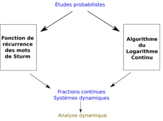
Figure 1: Le sch´ema de la th`ese.

Ici nous utilisons des outils propres aux systèmes dynamiques (comme l’opérateur de transfert) et au cadre de la combinatoire analytique [FS09]. La combinatoire analytique a pour objet fondamental les fonctions génératrices (ici de type “Dirichlet”, typiques de la théorie des nombres [Ten15]), avec des coefficients qui comptent des objets combinatoires (ou de théorie des nombres), et relie leur comportement analytique (les

(7)

6

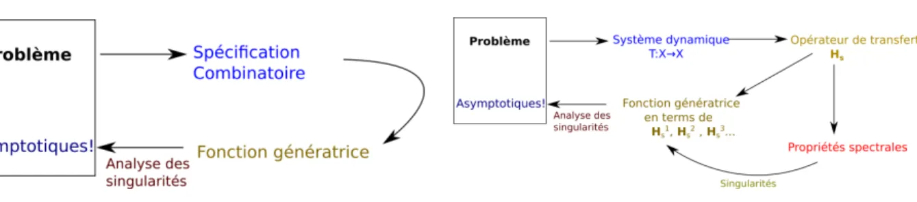
(a) Le flux de travail de la combinatoire analytique. (b) Le flux de travail de l’analyse dynamique.

Figure 2: La combinatoire analytique et son prolongement `a l’analyse dynamique.

singularités) aux asympytotiques de leur coefficients (grâce aux théorèmes tauberiens). La situation est illustrée dans la figure 2a. La combinatoire analytique est largement utilisée dans l’étude d’algorithmes, de structures de données, ou même en combinatoire per se, probabilistiquement. Quand les objets étudiés sont engendrés par un système dynamique, la combinatoire analytique peut (et doit) être complétée par une autre classe de méthodes, donnant lieu à ce qui s’appelle l’analyse dynamique [FV98], introduite par Baladi, Flajolet, Vallée et d’autres. L’outil clé de l’analyse dynamique est l’opérateur de transfert du système dynamique sous-jacent, qui étend l’opérateur transformateur de densité du système, et suit naturellement l’évolution de nos paramètres pendant l’itération du système. Nous pouvons alors utiliser cet opérateur pour engendrer des fonctions génératrices. Quand l’opérateur agit sur un espace fonctionnel approprié, il présente une valeur propre dominante, qui joue le rôle de la singularité dominante en combinatoire analytique. L’analyse dynamique est illustrée dans la figure 2b. Nous expliquons brièvement comment on y arrive. La puissance k-ième (par composition) de l’opérateur de transfert Hs décrit la situation après k iterations du système dynamique (sous-jacent à l’algorithme ou processus). Nous cherchons alors des expressions pour notre fonction génératrice en termes de puissances de Hs, souvent avec toutes les puissances appa-raissant en même temps (I − Hs)−1 = I + Hs+ H2s+ . . ., quand nous considérons toutes les exécutions possibles d’un algorithme. Trouver une telle expression peut parfois être impossible avec la combinatoire analytique classique, car l’utilisation des outils nécessite une certaine indépendence entre les différentes étapes de l’algorithme. Une fois que nous avons trouvé ces expressions pour les fonctions génératrices, nous utilisons les propriétés spectrales de l’opérateur; si l’opérateur a de bonnes propriétés (dans un espace fonctionnel approprié), l’action de la puissance Hk_s est déterminée par la valeur propre dominante et la pro-jectionsur l’espace propre associé. Par bonnes propriétés, nous entendons que l’opórateur présente un saut spectral[BV03] : la valeur propre dominante est unique et simple, et est séparée du reste du spectre. Nous remarquons que cette situation est similaire à celle du théorème de Perron-Frobenius pour des matrices; le comportement cherché est analogue mais dans un space de dimension infinie. Le choix de l’espace fonc-tionnel est délicat car il y a un compromisà trouver : l’espace doit être suffisamment grand pour contenir des fonctions utiles, mais suffisamment petit pour avoir un saut spectral. Une fois établi que les puissances de l’opérateur de transfert sont déterminées par les puissances de la valeur propre dominante, nous pouvons finir l’analyse et déterminer les singularités principales des fonctions génératrices.

´

Etude probabiliste des mots de Sturmian

Les mots de Sturm constituent une famille omniprésente en combinatoire des mots (voir e.g., [Fog02] et [Lot02]). Ce sont précisement les mots les plus simples qui ne sont pas ultimement périodiques, au sens qu’ils ont le plus petit nombre possible de facteurs de chaque longeur n, c’est-à-dire n+1. Les mots de Sturm apparaissent naturellement en relation avec la géométrie digitale et les quasicristaux, et, par conséquence, ont été beaucoup étudiés.

Sur l’alphabet binaire {0, 1}, Morse et Hedlund [MH40] fournissent une description arithmétique des mots de Sturm fondamentale, qui montre un lien profond avec les fractions continues. Plus précisément, ils

(8)

7

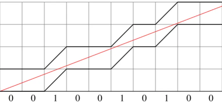
ont démontré qu’à chaque mot de Sturm correspond est associé un nombre irrationnel α de l’intervalle unité (appellé sa pente), qui décrit la fréquence des 1 dans le mot : chaque mot de Sturm peut être écrit systématiquement en fonction de sa pente comme Sα. Cette représentation correspond, en fait, à un codage discret de droite comme décrit dans la figure Figure 3.

0 0 1 0 0 1 0 1 0 0

Figure 3: Morse et Hedlund ont reli´e les mots de Sturm aux codages discrets de droites avec une pente irrationnelle α.

La fonction de récurrence du mot de Sturm Sα décrit la façon dont les facteurs finis de longueur n ar-rivent dans le mot infini Sα. En particulier, Rα(n) indique le “temps d’attente” maximum qu’il faut pour découvrir tous les facteurs de Sαde longueur n. La fonction Rα(n) dépend, d’une façon assez élégante, du couple (α, n). Plus précisément, Morse et Hedlund [MH40] ont relié la fonction de récurrence Rα(n) au dévelopepment en fraction continue de α, plus particulièrement à ses continuants qk(α), les dénominateurs des convergents de la fraction continue de α.

Morse and Hedlund ont démontré que, quand n appartient à l’intervalle [qk−1(α), qk(α)[ entre deux contin-uants consécutifs qk−1(α) et qk(α) de α, la fonction de récurrence Rα(n) admet une expression simple. De plus, les auteurs exhibent un comportement en “n log n” pour le pire cas de Rα(n), dont l’apparition dépend fortement du choix spécifique de (α, n), mais qui se produit presque sûrement pour une infinité de n. La question que nous posons est : Si le couple (α, n) est tiré au hasard de façon systématique, quel est le comportement probabiliste de la fonction de récurrence Rα(n)? Dans cette thèse, nous proposons deux modèles probabilistes différents pour répondre à la question.

Premier mod`ele probabiliste

Notre premier modèle, décrit dans le chapitre 5, a été publié en [BCR+15] pour la conférenceMFCS2015. C’est une première approche pour le pire cas d’un point de vue probabiliste obtenue en conditionnant avec des intervalles de plus en plus petits qui contiennent les pires cas. Dans ce modèle, nous tirons la pente α “uniformément” dans l’intervalle unité puis nous prenons de sous-suites particulières k →→ nkqui fixent la position barycentrique µ de n relative à l’intervalle [qk−1(α), qk(α)[. Nos résultats [BCR+15], obtenus par des méthodes d’analyse dynamique, quantifient l’incidence de la position µ sur le comportement du pire cas de la fonction de récurrence, et montrent effectivement un comportement du type “ n log n en moyenne” sur certaines sous-suites k →→ nk.

Nous utilisons des méthodes d’analyse dynamique, ici avec le système dynamique classique d’Euclide (avec l’application de Gauss) et son opérateur transformateur de densités. Nous démontrons que l’espérance associé à la k-ième étape nk s’écrit en termes de la puissance k-ième de l’opérateur transformateur de densités. Sur l’espace fonctionnel des fonctions de variation bornée, cet opérateur présente un saut spectral dont on a besoin, et les puissance de l’opérateur sont alors approchées par les (véritables) puissances de la valeur propre dominante. Dans ce cas nous avons eu besoin aussi de résultats sur le terme de reste, qui sont assez connus.

(9)

8

Deuxi`eme mod`ele probabiliste

Le modèle précédent est très utile quand il s’agit de décrire le pire cas de la fonction de récurrence et l’incidence de la position relative µ. Dans notre deuxième modèle nous considérons, à nouveau, une pente aléatoire α, mais la taille d’entrée n est fixée et indépendant de α. L’analyse de la fonction de récurrence dans ce modèle “n → ∞ fixé” est décrite au chapitre 4, et a été publiée dans les actes de ANALCO2017 [RV17]. Ce modèle peut être utilisé aussi afin d’étudier d’autres fonctions, comme la position relative µ, qui jouent un rôle dans l’analyse des mots de Sturm, ainsi que les fractions continues elles-mêmes.

Nous obtenons trois résultats principaux dans [RV17]; nous considérons les variables aléatoires α →→ (1/n)Rα(n) et les étudions pour n grand. Nous exhibons leur distribution limite, et nous démontrons l’existence de la densité limite. Nous étudions aussi l’espérance conditionnelle du quotient de récurrence

(1/n)Rα(n), quand nous excluons la possibilité que n se trouve trop proche du bord gauche de l’intervalle [qk−1(α), qk(α)[. Enfin, nous exhibons une classe d’événements pour lesquels l’ordre de cette espérance conditionnelle est exactement log n. Ce dernier résultat peut être considéré comme une extension proba-biliste du résultat classique de Morse et Hedlund.

Nos preuves utilisent des méthodes élémentaires : elles reposent sur une comparaison précise entre une intégrale et sa somme de Riemann; cependant, l’intégrale est impropre (mais convergente) et la somme de Riemann implique une condition supplémentaire de primalité, ce que nous avons appellé une “somme de Riemann première”. Les sommes de Riemann premières apparaissent aussi dans [BCZ03], où les auteurs étudient la suite de Farey, mais travaillent dans des domains bornés. Ici nous adaptons les méthodes pour des domaines non bornés, avec des termes d’erreur précis pour la convergence vers les intégrales.

Comportement probabiliste de familles “particuli`eres” de mots de Sturm

Il y a deux familles particulières de mots de Sturm qui sont importantes en tant que telles. Leur étude constitue un travail un cours qui, en fait, vise à unifier les approches pour les deux familles et le cas générique du deuxième modèle. Nos résultats actuels (non encore publiés) montrent que le comportement de ces familles est semblable au cas générique. Les preuves utilisent aussi d’autres outils utiles tels que les séries de Dirichlet et les théorèmes taubériens.

Christoffel words Quand la pente α est rationnelle, le mot Sαest périodique, ce que l’on appelle un mot de Christoffel [BLRS08]. Dans ce cas, la question est : Est-ce vrai que, quand la longueur du développement en fraction continue d’α tend vers l’infini, la fonction de récurrence a un comportement en moyenne semblable à celui d’un mot de Sturm générique?

Mots de Sturm engendrés par morphisms Il y a une deuxième famille importante, à savoir, les mots de Sturm qui sont engendrés par de morphisms [All98]. Ils sont associés à des pentes α irrationnelles quadratiques, qui ont des développements en fractions continues périodiques. Ici nous posons une question similaire : Est-ce vrai que, quand la période de l’irrationnel quadratique α tend vers l’infini, le comporte-ment de la fonction de récurrence, en moyenne, est semblable à celui du cas générique? L’analyse dans ce cadre est plus compliquée car elle dépend de (n, α, ℓ) où ℓ dénote la quantité de tours de la période.

Analysis of the Continued Logarithm Algorithm

L’algorithme du logarithme continu –CL pour ses initiales en anglais– est introduite par Gosper dans Hak-mem [Gos78] comme une “mutation” de l’algorithme classique des fractions continues. Cet algorithme

(10)

9

calcule le plus grand commun diviseur de deux nombres entiers en utilisant uniquement des shifts binaires et des soustractions. Le pire cas a été étudié récemment par Shallit [Sha16], qui a donné des bornes précises pour le nombre d’étapes et a exhibé une famille d’entrées sur laquelle l’algorithme atteint cette borne. Dans cete thèse, nous étudions le nombre moyen d’étapes, tout comme d’autres paramètres importants de l’algorithme. Grâce à des méthodes d’analyse dynamique, nous exhibons des constantes mathématiques précises.

Plus précisément, nous considérons les couples (p, q), avec 1 ≤ p ≤ q ≤ N , avec la probabilité uniforme, et nous étudions les valeurs moyennes du nombre d’étapes de pseudo-divisons et de shifts binaires, quand N → ∞. Dans notre résultat principal, le théorème 7.2, nous démontrons que ces valeurs moyennes sont asymptotiquement linéaires par rapport à la taille log N , et nous décrivons précisement leur comportement asymptotique quand N → ∞.

Le système dynamique sous-jacent ressemble à première vue à celui d’Euclide, et a été étudié d’abord par Chan [Cha05] et Borwein et al [BCLM17], avec des méthodes ergodiques, mais la présence des puis-sances de 2 dans les quotients change la nature de l’algorithme et donne une nature dyadique aux principaux paramètres de l’algorithme, qui ne peuvent donc pas être simplement caractérisés dans le monde réel. C’est pourquoi nous introduisons un nouveau système dynamique, avec une nouvelle composante dyadique, et tra-vaillons dans ce système à deux composantes, l’une réelle, et l’autre dyadique. Grâce à ce nouveau système mixte, nous obtenons l’analyse en moyenne de l’algorithme.

(11)

10

Acknowledgements. I begin by thanking my thesis directors. First Alfredo Viola, who has uncondition-ally supported me since the times of the “Low-correlation sequences” seminar and introduced me to my other thesis directors Valérie Berthé, Brigitte Vallée, as well as the community in general. I keep very fond memories of our time together and hope we will continue to have seminars or work discussions for a long time. I am profoundly grateful to Brigitte, who has helped me and taught me a lot, through her seemingly unbounded energy. We have worked a lot together, and I think that, even though we have had our share of divergence and communication problems, overall it has been very positive and led to interesting and unex-pected ideas (in part due to this divergence of thought process!). I would like to thank Valérie, who has always supported me, both academically and administratively, and directed me towards interesting topics and problems which resulted in this thesis. I hope we can continue to work on the pending topics and unify it with the rest of the work.

I would like to express my gratitude to the referees, Bruno Salvy and Pierre Arnoux, for having accepted to review my thesis through the summer, and for all of their corrections and suggestions. They have certainly helped improve the quality of this dissertation. I also extend my thanks to all of the members of the jury for having accepted to be here for my defence, I feel honoured.

I thank the whole IRIF, the PhD students, the ATERs and everyone that has made me feel welcome. Heartfelt thanks go to the people from the AMACC team in Caen, Ali, Julien, Lo¨ıck, as well as Eda Cesaratto from Universidad Nacional de General Sarmiento, for the useful discussions, work and seminars enjoyed together. I thank the secretaries from GREYC in Caen, who have helped me with various “missions”.

My sincere thanks to Alberto Pardo and Franco Robledo, from Universidad de la Rep´ublica, as well as the secretary Mar´ıa In´es, who have made the cotutelle possible.

My research would have been impossible without the funding from the ANR DynA3S.

Finally, I want to thank my family, my friends, both from Uruguay, from the Maison de l’Italie and IRIF, for their constant support.

(12)

INTRODUCTION

General context

In this dissertation, we study objects coming from a priori diverse fields: first, a very important family of words, the so-called Sturmian words, fundamental in Combinatorics on Words; second, a gcd algorithm (the Continued Logarithm Algorithm – CL for short), stemming from Number Theory. These objects have been studied extensively, and the “extreme orders” of some of their important characteristics are now well-understood. We adopt a different point of view; we wish to study them from a probabilistic perspective. Rather than being motivated the question “what is the worst/best case scenario?”, we consider questions such as “what does a random (Sturmian) word look like? what does a random gcd algorithm execution look like ?

Even though the objects we consider (words, gcd algorithms) come from seemingly distant fields, they can both be described within a common Number Theoretic framework. This framework includes continued fraction expansions (the usual one for Sturmian words, and a less classical one for the CL algorithm, where powers of two play a central role), and their corresponding underlying dynamical systems.

Figure 4: The diagram of this thesis.

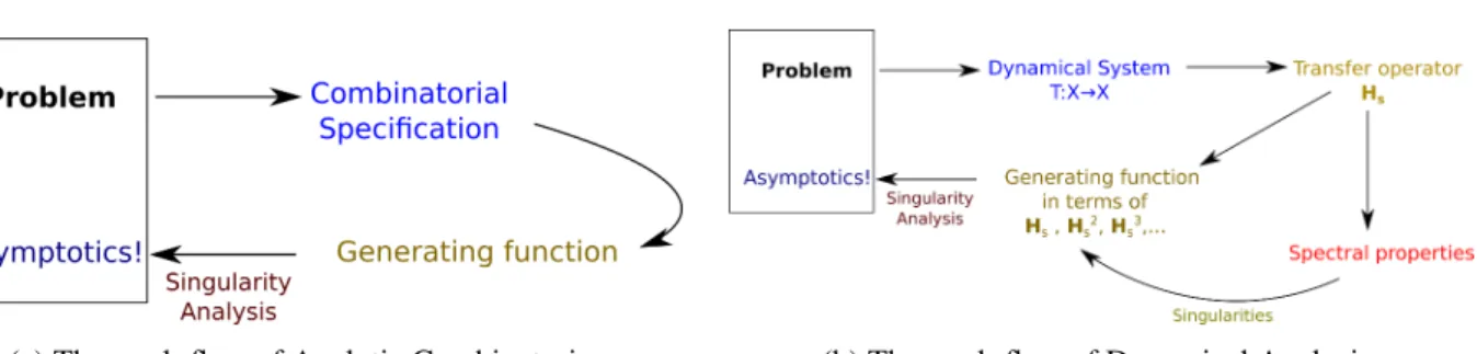
Here we apply techniques originating from Analytic Combinatorics and Dynamical Systems. Analytic Com-binatorics [FS09] deals with generating functions (here of Dirichlet type, stemming from Number Theory [Ten15]), with coefficients counting combinatorial (number theoretical) objects, and relates their analytic behavior (notably their singularities) to the asymptotics of their coefficients (here via Tauberian Theorems). The situation is illustrated in Figure 5a. Analytic Combinatorics is widely used to study algorithms, data structures, or combinatorial objects per se, probabilistically. When the objects of interest are generated by a

(17)

CONTENTS 16

(a) The work-flow of Analytic Combinatorics. (b) The work-flow of Dynamical Analysis.

Figure 5: Analytic Combinatorics and the extension to Dynamical Analysis.

dynamical system, Analytic Combinatorics can be (and must be) complemented by another class of methods, giving rise to the so-called Dynamical Analysis [FV98], pioneered by Baladi, Flajolet, Vall´ee and others. The key object in Dynamical Analysis is the transfer operator of the underlying dynamical system, which extends the density transformer operator of the system, and naturally tracks the evolution of our parameters of interest through its iterates. It thus can be viewed as a generating operator that generates itself the gen-erating functions of interest. When it acts on a convenient functional space, this operator has a dominant eigenvalue, which plays the same role as the dominant singularity in classical Analytic Combinatorics. The extension to Dynamical Analysis is illustrated in Figure 5b. We briefly explain how this is achieved. The k-th power (by composition) of the transfer operator Hsreflects the situation after k iterations of the dynamical system (underlying the algorithm or process). Thus we must first exploit this to give expressions for our target generating functions in terms of the powers of Hs, often with all powers at the same time (I − Hs)−1 = I + Hs+ H2s+ . . . when considering every possible execution of an algorithm. Finding such an expression is sometimes impossible in classical Analytic Combinatorics, as the usual techniques require some sort of independence between distinct steps of the algorithm. Given expressions for our generating functions in terms of the powers of Hs, we exploit the spectral properties of the operator; if the operator is well-behaved (in an appropriately chosen functional space), the action of the power Hk_s is determined by the dominant eigenvalue and the projection over its eigenspace. By well-behaved we mean it presents a spectral gap [BV03]: the dominant eigenvalue is unique and simple, and separated from the rest of the spectrum. The reader may be familiar with the Perron-Frobenius Theorem for matrices; the target behavior is analog but in a space of infinite dimension. The choice of the functional space is then a delicate one as there must be a balance: it must be big enough to contain useful input functions, but small enough to give us our desired spectral gap. Then, once we have established that the powers of the operator follow the powers of the dominant eigenvalue, we may complete the analysis and determine the main singularities of the generating functions.

This dissertation is structured into 3 parts, following the bottom of the diamond in Figure 4:

• Part I is concerned with the common background for the whole thesis, which corresponds to the bottom part of Figure 4. We introduce the background in continued fractions and dynamical systems in Chapter 1. Particular attention has been payed to introducing continued fractions, dynamical systems and the functional properties of the transfer operator. The concepts we require from Analytic Combinatorics are introduced in Chapter 2, in particular Dirichlet Generating Functions and the Tauberian Theorem.

• Part II deals with the problems coming from Combinatorics on Words. Therein we define all the necessary notions concerning Sturmian words and our problematic (in Chapter 3), to then proceed to our probabilistic study of Sturmian words (in chapters 4 and 5).

• Finally, Part III closes the thesis with a probabilistic study of the CL algorithm. Now we give further details regarding the contents of Part II and Part III.

(18)

CONTENTS 17

Probabilistic study of Sturmian words

Sturmian words are central objects in Word Combinatorics (see e.g., [Fog02] and [Lot02]). These are precisely the simplest infinite words that are not eventually periodic, in the sense that they have the absolutely smallest number of factors of each length n, that is n + 1. Sturmian words turn up naturally in relation to digital geometry and quasicrystals, and have been widely studied.

On the binary alphabet {0, 1}, Morse and Hedlund [MH40] provide a powerful arithmetic description of Sturmian words and relate them to continued fraction expansions. Specifically, they show that each Sturmian word is in strong correspondence with an irrational number α of the unit interval (called its slope), describing the frequency of ones in the word: each Sturmian word may be written as Sα for some irrational α in the unit interval. This representation is related to the discrete coding of lines such as the one in Figure 6.

0 0 1 0 0 1 0 1 0 0

Figure 6: Morse and Hedlund connected Sturmian words to discretized lines of irrational slope α. The recurrence function of the Sturmian word Sα describes how the finite factors of length n occur inside the infinite word Sα. In particular Rα(n) denotes the maximum “waiting time” that is needed to discover all the factors of Sαof length n. The function Rα(n) depends nicely upon the pair (α, n). More precisely, Morse and Hedlund [MH40] relate the recurrence function Rα(n) to the continued fraction expansion of α, more particularly to its continuants qk(α), the denominators resulting from the convergents of the continued fraction for α.

Morse and Hedlund showed that when n belongs to the interval [qk−1(α), qk(α)) between two consecutive continuants qk−1(α) and qk(α) of α, the recurrence function Rα(n) admits a simple expression. Further, the authors exhibited a “n log n” worst-case behavior for Rα(n), whose occurrence depends strongly on the specific choices of (α, n), but occurs almost surely for infinitely many n.

We present the general background regarding Sturmian words as well as Morse and Hedlund’s results, rewritten in our notation, in Chapter 3. We deemed, in particular, that the link between the recurrence of Sturmian words and continuants had to be explained thoroughly as we make extensive use of it. Finally, at the end of the chapter, in Section 3.4, we discuss Morse and Hedlund’s classical results concerning the growth of the recurrence function and we present briefly our context, questions, and results.

The question we pose is: If the pair (α, n) is chosen randomly in some systematic way. What is the prob-abilistic behavior of the recurrence functionRα(n)? In this dissertation, we consider two distinct proba-bilistic models to answer this question. Roughly speaking, our first model [BCR+15] considers sequences of n, appropriately chosen for each α, in turn chosen uniformly at random, while our second model [RV17] leaves n fixed and large (n → ∞) and chooses α at random. The latter is described and studied in Chapter 4 while the former in Chapter 5, and the relation between the two models is studied in Chapter 6. For each model, we answer the preceding question by giving precise limit distributions and densities, and studying how these relate to the worst-case “n log n” behavior, found by Morse and Hedlund, through the study of appropriate conditional probabilities.

(19)

CONTENTS 18

First probabilistic model

Our first model, described in Chapter 5, was published in [BCR+15] forMFCS 2015. It was a first attempt to approach this worst-case scenario from a probabilistic setting by actually conditioning to smaller and smaller sets which encapsulate the worst cases. In this setting, one picks the slope α “uniformly at random” from the unit interval and then considers particular subsequences k →→ nk that fix the barycentric position µ of n within the interval [qk−1(α), qk(α)). Our results in [BCR+15] , following a Dynamical Analysis, quantify the incidence of the position µ on the worst-case behavior of the recurrence function, and exhibit a “ n log n average behavior” over certain sequences k →→ nk.

More precisely, we exhibit the asymptotic value, as k → ∞, of the distribution of(1/nk)Rαnk



. As this analysis may be performed even for varying relative position µk, we show a kind of Morse-Hedlund result “on average”: the expectation is of order n log n when µk → 0 at a prescribed exponential rate.

Considering the dynamical system underlying the problem (here the classical Euclidean one, with the Gauss map), we use methods from Dynamical Analysis, in this case the plain density transformer operator of the system. We express the expectations relative to the k-th step in terms of the k-th power of the density transformer. Over an appropriate functional space (here the functions of bounded variation), the operator presents our desired spectral gap, and the powers of the operator are approximated by the (true) k-th power of the dominant eigenvalue. In this case we also require specific knowledge regarding the remainder term, which has been studied extensively for the Euclidean system.

Main results for the first probabilistic model. The main results obtained are summarized here:

▷ Theorem 5.1. For a fixed relative (barycentric) position µ , we characterize the limit expectations and the limit density of (1/nk)Rα(nk) as k → ∞.

▷ Theorem 5.2. For a varying relative (barycentric) position µk → 0 , we characterize the the limit density of (1/nk)Rα(nk) as k → ∞, demonstrating the rate of convergence to the case of fixed µ = 0 from Theorem 5.1. Moreover, we demonstrate that the expectations of (1/nk)Rα(nk) do have a log nkbehavior when µktends to zero exponentially (not too fast).

Second probabilistic model

The previous model for Sturmian words is very useful when it comes to describing the worst-case behavior of the recurrence function and the incidence of the relative position µ. Our second model considers, again, a random slope α, but somewhat orthogonally to the previous model, we take an input size n independent from α. The analysis of the recurrence function within this “fixed n → ∞” model is described in Chapter 4, and was published in the proceedings of ANALCO 2017 [RV17]. This model can be employed to study other functions, such as the relative position µ, playing a role in the analysis of Sturmian words, or continued fractions.

We obtain three main results in [RV17]; we consider the random variables α →→ (1/n)Rα(n) and study them for large n. We exhibit a limit for their distribution, and prove the existence of a limit density. We also study the conditional expectation of the recurrence quotient(1/n)Rα(n), when we exclude the possibility that n be too close to the left-end of the interval [qk−1(α), qk(α)). Finally, we describe a class of events for which the order of this conditional mean value is exactly of order log n. This can be viewed as a probabilistic extension of the Morse and Hedlund result.

Our proofs use elementary methods: they are based on a precise comparison between an integral and its Riemann sum ; however, the integral is improper (but convergent) and the Riemann sum is constrained by a coprimality condition, what we call a “coprime Riemann sum”. Coprime Riemann sums appear in [BCZ03],

(20)

CONTENTS 19

where the authors study the Farey sequence, but limited to bounded domains. Here we adapt the methods of proof to unbounded domains, getting tight error bounds for the convergence towards the integrals.

We introduce a general family of functions, called continuant-functions or Q-functions, which are defined via the sequence of continuants k →→ qk(α). Ustinov in [Ust09] had already considered similar functions to answer a question from Sinai and Ulcigrai [SU08]; here we generalize the class of functions to Q-functions, demonstrating its ubiquity in continued fraction problems. The recurrence quotient(1/n)Rα(n) is an instance of this family, and the other “geometric” parameters of interest provide natural examples of such a notion. The class of Q-functions lead naturally to coprime Riemann sums. Thus the paper describes a framework for studying the more general Q-functions, giving special attention to the recurrence function.

Main results for the second probabilistic model. The main results obtained are summarized here: ▷ Theorem 4.1. We show that for a wide family of Q-functions, which we call LQ-functions, the random variables (1/n)Rα(n) have a limiting distribution as n → ∞. This distribution is expressed in terms of an analog ψ(x, y) of the Gauss measure. Moreover, we show explicit bounds for the remainder term.

▷ Theorem 4.2. This result makes precise when the histograms do converge to the derivative of the distri-bution, thus making sense of it as a density. Since the distributions of Q-functions, such as (1/n)Rα(n), are discrete, we have to be careful when speaking of the limit density. Here we characterize this limit density of LQ-functions completely, giving also remainder terms.

▷ Theorem 4.3. This result demonstrates that if we condition to an event such as µ ≥ ϵ(n), which pre-vents that n be too close to the left-end of the interval [qk−1(α), qk(α)), the expected value of (1/n)Rα(n) involves a log ϵ(n). This is the counter-part of the results by Morse and Hedlund for this probabilistic model. The proof exploits strongly the knowledge of the remainder term from Theorem 4.1.

We highlight also that the convergence in distribution for Q-functions still holds for more general conditions, but without any guarantee for the remainder term however, see Theorem 4.10.

Probabilistic behavior of “particular” Sturmian words

There are two kinds of special Sturmian words, both interesting in their own right.

Christoffel words When the parameter α is rational, the word Sα is periodic and is called a Christoffel word [BLRS08]. It is still interesting to study such words probabilistically, particularly how the word evolves (when the length p(α) of its continued fraction becomes large) towards a Sturmian word, notably from the point of view of its recurrence function. Our main question is: Is it true that, when the length of the continued fraction ofα becomes large, the behavior of the recurrence function becomes close to the recurrence function of a generic Sturmian word?

We have carried out this study, yielding results in the same vein as the ANALCO paper. This results are

not yet published, and we explain them in subsection 6.3.1. We consider the set ΩN of rational numbers from the unit interval with a denominator at most N , endowed with the uniform probability. We introduce generating functions of Dirichlet kind, in order to sieve the right rationals for our asymptotics (through a Tauberian Theorem). We show that when the bound for the denominator N tends to infinity, the analogous distributions for the recurrence quotient are given by the same coprime Riemann-sum as before.

Sturmian words generated by morphisms There is a second important family of Sturmian words, namely Sturmian words that are generated by word morphisms [All98]. They are associated to quadratic irrationals α, that give rise to periodic continued fraction expansions. Our main question is: Is it true that, when the

(21)

CONTENTS 20

periodπ(α) of the quadratic irrational α becomes large, the behavior of the recurrence function resembles that of a generic Sturmian word?The analysis is more difficult because it now depends on the triple (n, α, ℓ) where the integer ℓ describes the number of times the period is needed.

We have already obtained interesting results for the case ℓ = 1 (not yet published), where we get the same distributions from our second probabilistic model but through substantially different methods. There seems to be a stationary behavior as ℓ → ∞, and this is work still in progress. The results obtained thus far are discussed in subsection 6.3.2.

Our proofs mix methods from dynamical analysis and elementary methods like those in the second model: as for rational numbers, we introduce generating functions of Dirichlet type to manage the quadratic irra-tionals, which are endowed with their usual notion of size, here closely related to the fundamental unit of the associated quadratic field. The associated generating functions are (again) expressed in terms of the transfer operator of the Euclid dynamical system, but now via their traces. This leads to a more involved study.

A specific interesting result This study also leads us to a specific interesting result on finite continued frac-tions. Such a continued fraction is defined by a finite sequence (m1, m2, . . . mk) of partial quotients and rep-resents a rational p/q. The “mirror” continued fraction defined by the mirror sequence (mk, mk−1, . . . m1) represents another reduced rational p′/q that has the same denominator as the previous one (but not the same numerator). Very often, the two expansions occur together in our studies (and in many other studies), and the two associated rational numbers seem a priori to be correlated in a strong way. We adapt a result of Shparlinski [Shp12, Theorem 13] and we prove that, when one draws a rational p/q uniformly at random, the two rational numbers p/q and p′/q asymptotically behave in an independent way, as the denominator q becomes large. This is explained in Section 4.5.3.

Analysis of the Continued Logarithm Algorithm

The Continued Logarithm Algorithm –CL for short– introduced by Gosper in 1978 [Gos78], computes the gcd of two integers; it employs efficient operations, as it only performs (binary) shifts and subtractions. Shallit [Sha16] has studied its worst-case complexity in 2016 and showed it to be linear, and he proposed the problem of determining the average-case analysis of the algorithm to us. We answer his question in the publication [RVV18], accepted inLATIN 2018 and described in Chapter 7: we study its main parameters (number of iterations K, total number of shifts S) and obtain precise asymptotics for their mean values. More precisely, we consider the set ΩN gathering all integer pairs (p, q) with 1 ≤ p ≤ q ≤ N , endowed with the uniform probability, and we study the mean values of K and S as N → ∞. In our main result, Theorem 7.2, we prove that these mean values are asymptotically linear in the size log N , and describe precisely their asymptotic behavior as N → ∞. This result is to be expected intuitively, since the algorithm resembles the Euclidean one where both the worst and average case are linear [Val06]. The study leading up to this average case asymptotics, however, presents several interesting (and non-trivial) aspects.

The dynamical analysis involves the dynamical system underlying the algorithm, which produces continued fraction expansions whose quotients are powers of 2. Even though this CL system has already been studied by Chan [Cha05] and Borwein et al [BCLM17], the presence of powers of 2 in the quotients ingrains into the central parameters a dyadic flavor that cannot be grasped solely by studying the CL system. Indeed, even if the input of the CL algorithm is a pair of coprime integers, the algorithm builds a sequence qkof remainders, for which the pair (qk−1, qk) is no longer coprime. The successive gcd(qk−1, qk) are now powers of 2, and it appears experimentally that (1/k) log₂gcd(qk−1, qk) gets close to 1/2 as k becomes large.

In order to take into account this involved dyadic phenomenon, central to our analysis, we add a second dyadic component to the (usual) CL dynamical system, and work with a two-component system, which

(22)

CONTENTS 21

allows us to keep track of all the interesting parameters under study. This new dynamical system with its two components, is not classical at all, but we succeed in finding a convenient space where its transfer operator acts nicely, with a single dominant eigenvalue. With this new mixed system at hand, we provide a complete average-case analysis of the CL algorithm, with explicit constants.

The extended dynamical system and its properties are presented in Section 7.4. In particular, in Section 7.4.2 we discuss to a certain extent the appropriate probability measures on the dyadics, while in Section 7.4.3 we provide the properties of the transfer operator that are needed to complete the analysis. This becomes significant because the use of dyadics in Dynamical Analysis performed here is not commonplace. Even though there exist works studying other gcd algorithms that employ dyadics, namely the so-called “Turtle and the Hare” algorithm [DMDV05], and the Binary algorithm [Val98a] , the CL algorithm evolves and uses the dyadics in a novel way.

Main results for the CL algorithm. The main result obtained is summarized here:

▷ Theorem 7.2. The mean value of the total number of iterations K and the total number of shifts S are asymptotically linear in the size log N as N → ∞, and we provide explicit constants.

We remark that we are working on the so-called “real case” for the Continued Logarithm expansion. We consider a random real in the unit interval and, a given number k, we wish to describe the evolution of the main parameters associated with the expansion truncated after k steps, when the depth k tends to ∞. This is a work still in progress.

(23)

(24)

Part I

Presentation of the general context

(25)

(26)

CHAPTER 1 CONTINUED FRACTIONS AND THE

GAUSS MAP

We kick off by introducing several useful concepts that are recurrent in our studies and will prove funda-mental for both the solution and conception of our problems.

1.1 The numeration process

Continued fractions can be introduced in several ways, and arise in contexts as seemingly diverse as dio-phantine approximation and Pell’s equation. The most classical text describing extensively the elementary properties of continued fractions is definitely “Continued Fractions” by Khinchin [Khi97].

A continued fraction is a “formal” expression of the form 1 m1+ 1 m2+ 1 m3+. .. ,

which we denote by [m1, m2, . . .], where the coefficients m1, m2, . . ., known as quotients or partial quo-tients, are positive integers.

We can make sense of this as a limit of the so-called convergents [m1, . . . , mk] := 1 m1+ 1 . .. + 1 mk , (1.1)

that is, the truncated expansion considering only the first k coefficients. This can be realized as a finite continued fraction, or by filling in with 0s as follows [m1, . . . , mk, 0, 0, 0 . . .], thus explaining the notation. More precisely define

[m1, m2, . . .] := lim[m1, . . . , mk] , 25

(27)

1.1. THE NUMERATION PROCESS 26

and this limit is well-defined (see e.g., [Khi97]) , for any choice of quotients m1, m2, . . . ≥ 1. We will now describe how of the continuants evolve, and in fact derive the existence of the limits too, as well as other interesting properties.

The finite continued fraction [m1, . . . , mk] represents a rational number pk qk = 1 m1+ 1 . .. + 1 mk , gcd(pk, qk) = 1 , (1.2)

where we enforce that pkand qkto be coprime to make the choice unique.

Note pk and qk defined in (1.2) depend only on the vector (m1, . . . , mk) ∈ Zk≥1 and hence we will often write p(m1, . . . , mk) and q(m1, . . . , mk) to underline this dependence, or even pk(m) and qk(m) when the whole sequence m = (m1, . . . , mk, . . .) is fixed beforehand, thus emphasizing the “truncation” aspect. We write simply pkand qkas above when there is no danger of confusion.

The limit [m1, m2, . . .] in (1.1) actually exists for any choice of coefficients (mk)∞_k=1 (this is proved e.g., in [Khi97, Theorem 10, p.10]) and represents a real number α ∈ [0, 1]. Conversely, every real number α ∈ (0, 1] has a continued fraction expansion

α = 1

m1+ 1 m2+. ..

, (1.3)

and we write mi= mi(α) when there is danger of confusion. This expansion is unique when α is irrational and, of course, necessarily infinite. For rationals we have two expansions, both finite (we will point out why later on), by means of the equality

[m1, . . . , mk−1, mk] = [m1, . . . , mk−1, mk− 1, 1] (1.4) which holds for mk≥ 2.

Thus rationals have two finite expansions; one of them ending with the digit 1. It is direct to see that this is the only possible “redundancy” in the continued fraction expansion (this can be seen by direct comparisons), somewhat analogously to the case of the binary base representation, where the redundancies come from the cases of the form 0.a1. . . ak100 . . . = 0.a1. . . ak011 . . . This is to say, if two continued fraction expansions represent the same real number, then we are necessarily in the case (1.4) described above.

When considering the quotients m1(α), m2(α), . . . coming from the expansion of α, we will also write pk(α) and qk(α) to denote the numerators and denominators of the convergents. The sequence (qk(α))∞_k=1 of denominators is known as the sequence of continuants, and plays a fundamental role in our studies. Given α ∈ (0, 1) it will be useful to explain how its expansion is computed. We first note that if equality (1.3) is to hold, then

1

α = m1+ [m2, m3, . . .] which implies m1(α) =

₁

α, where ⌊·⌋ denotes the floor function. Then the continued fraction [m2, m3, . . .] corresponds, in its turn, to the rational part {1/α} and the procedure is iterated.

Thus we may think of this procedure as a dynamical system producing the digits m1(α), m2(α), . . .

1.1.1 The Gauss map

The process of computing a continued fraction expansion, its successive digits, can be described somewhat more.

(28)

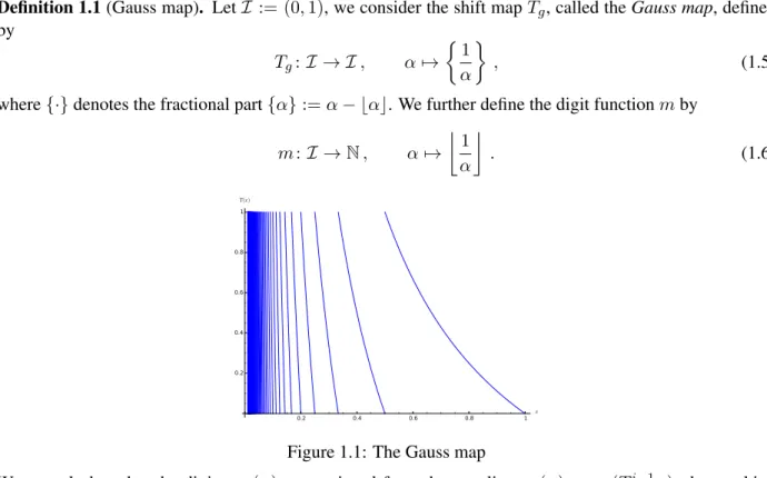
Definition 1.1 (Gauss map). Let I := (0, 1), we consider the shift map Tg, called the Gauss map, defined by Tg: I → I , α →→  1 α  , (1.5)

where {·} denotes the fractional part {α} := α − ⌊α⌋. We further define the digit function m by m : I → N , α →→ 1 α  . (1.6) 0.2 0.4 0.6 0.8 1 x 0.2 0.4 0.6 0.8 1 T(x)

Figure 1.1: The Gauss map

We remark then that the digits mi(α) are retrieved from the equality mi(α) = m(Tgi−1α), thus making the continued fraction expansion a coding of the trajectory {α, Tgα, Tg2α, . . .} by m. Note that this is well defined when α ∈ I \ Q, while the trajectory will be finite when α is rational, as we will soon explain. The evolution of the orbits through the Gauss map Tgfrom Definition 1.1 constitutes a fundamental example in dynamical systems. We extend the notions given for the Gauss map to more general dynamical systems in Section 1.2, where we define complete interval dynamical systems in Definition 1.3.

Observation 1.1. It is important to remark that the Gauss map Tg and the digit function m are defined so that

α = 1

m1(α) + Tg(α)

. (1.7)

This equation may be iterated giving

α = 1 m1(α) + 1 . .. + 1 mk(α) + Tgkα , (1.8)

which we denote by [m1(α), m2(α), . . . , mk−1(α), mk(α) + Tgkα] in a little abuse of notation (as we are introducing non-integer coefficients).

1.1.2 Continued fractions and the Euclidean Algorithm

The Euclidean Algorithm computes the greatest common divisor (gcd) of a pair of positive integers a ≤ b by exploiting the equality gcd(a, b) = gcd(r, a) where r = b mod a is the remainder of the division of b by a, and then proceeding likewise with (r, a) until we get to a pair (0, g) for which it is clear that gcd(0, g) = g. This algorithm is very efficient, having linear complexity (on the bit-length) of a and b. Here we explain this fact briefly, by showing that there is a fundamental connection between the Euclidean Algorithm and continued fractions of rational numbers.

(29)

Continued fractions are naturally equivalent to the execution of the Euclidean algorithm. Indeed, let us pick a rational number a/b. One step of the expansion gives:

a b = 1 b/a = 1 ⌊b/a⌋ + {b/a},

and here {b/a} = b mod a_a so that our original pair (a, b) has become (b mod a, a) after one iteration, exactly like in the Euclidean Algorithm. As we know, the Euclidean algorithm certainly terminates, as the first entry always decreases strictly until becoming 0 (clearly b mod a < a), thus giving a finite representation

a b = 1 m1+ 1 . .. + 1 mk ,

where m1, m2, . . . are the quotients of the divisions in the Euclidean algorithm applied to (a, b)!

In particular, as (1.4) is the only redundancy in the representation, rational numbers have only finite expan-sions (exactly two of them). Second, this means that one may study the Euclidean algorithm by studying the continued fraction expansion or viceversa.

1.1.3 Basic properties of continuants

We now develop important properties regarding the convergents pk/qk, providing information regarding the growth of the sequence of continuants qk. These will prove useful in proving that α = [m1(α), m2(α), . . .] indeed holds as expected, as the convergence rate of [m1(α), m2(α), . . . , mk(α)] towards α will be dictated by the size of qkas we explain in Proposition 1.4. Along the way we will introduce several properties which are fundamental to our studies.

We start off by studying the recurrence equation satisfied by the sequences (pk)k and (qk)k, providing its matricial form too.

Proposition 1.1. Let (mk)∞_k=1 be a sequence of positive integers. The sequences (pk)∞_k=1 ⊂ N and (qk)∞k=1 ⊂ N of successive numerators and denominators of the continued fraction expansion, defined by

pk qk

= [m1, . . . , mk] , gcd(pk, qk) = 1 , satisfy the recurrences

pk+1= mk+1pk+ pk−1, qk+1 = mk+1qk+ qk−1, (1.9) for allk ≥ 0, where we consider p0 = 0, p−1= 1 and q0= 1, q−1 = 0.

This can be written in matricial form as qk+1 pk+1 qk pk  =mk+1 1 1 0   qk pk qk−1 pk−1  , (1.10) along with  q0 p0 q−1 p−1  =1 0 0 1  . (1.11)

Proof. For convenience will prove the proposition in matricial form. Observe that the result is equivalent to  q(m1, . . . , mk) p(m1, . . . , mk) q(m1, . . . , mk−1) p(m1, . . . , mk−1)  =mk 1 1 0  · · ·m1 1 1 0  , (1.12)

(30)

for all k ≥ 0 and (m1, . . . , mk) ∈ Nk. This expression is particularly useful as what we effectively do in the inductive step is add the coefficient m1to the beginning of (m2, . . . , mk) ∈ Nk, for which we assume the result to hold by induction.

The proof proceeds by strong induction over k. It is clear that the base case p0 = 0, p−1 = 1 and q0 = 1, q−1 = 0 holds for any choice of the quotients. Now assume that the recurrence holds for j up to k, for any choice of quotients m1, . . . , mk(strong induction). Let us consider now a concrete m1, . . . , mk, mk+1 and show (1.12) for tuple of length k + 1.

We have p(m1, . . . , mk+1) q(m1, . . . , mk+1) = 1 m1+p(m_q(m2₂,...,m_,...,mk+1_k+1₎) = q(m2, . . . , mk+1) m1q(m2, . . . , mk+1) + p(m2, . . . , mk+1) ,

and therefore p(m1, . . . , mk+1) = q(m2, . . . , mk+1) as well as q(m1, . . . , mk+1) = m1q(m2, . . . , mk+1)+ p(m2, . . . , mk+1) because their gcd equals gcd(q(m2, . . . , mk+1), p(m2, . . . , mk+1)) = 1 .

As the previous equalities will also hold when we substitute k →→ k − 1, we have q(m1, . . . , mk+1) p(m1, . . . , mk+1) q(m1, . . . , mk) p(m1, . . . , mk)  =q(m2, . . . , mk+1) p(m2, . . . , mk+1) q(m2, . . . , mk) p(m2, . . . , mk)  m1 1 1 0  .

It follows from the inductive hypothesis that

q(m2, . . . , mk+1) p(m2, . . . , mk+1) q(m2, . . . , mk) p(m2, . . . , mk)  =mk+1 1 1 0  · · ·m2 1 1 0  , thus q(m1, . . . , mk+1) p(m1, . . . , mk+1) q(m1, . . . , mk) p(m1, . . . , mk)  =mk+1 1 1 0  · · ·m2 1 1 0  m1 1 1 0  ,

which proves the result for k + 1. ■

An immediate corollary of the recurrence is that the sequence of continuants grows at least exponentially. Corollary 1.1. Let (mk)∞k=1be a sequence of positive integers. The sequence(qk)∞k=1 ⊂ N of successive continuants of the continued fraction expansion satisfies

qk≥ 2(k−1)/2.

Proof. Observe that qk+1≥ 2qk−1by the recurrence. ■

Observation 1.2 (Precise bound). This last inequality can be made somewhat more precise by considering that qk+1≥ qk+ qk−1. Then by induction we conclude that qk ≥ fkwhere fkis the k-th Fibonacci number, defined from f0 = 0, f1 = 1 and fj+1 = fj + fj−1 for j ≥ 1. Equality can only hold for each k if α = [1, 1, 1, . . .] which then satisfies α = 1/(1 + α) so that α = (√5 − 1)/2.

Finally, we recall that fk = ⌊Φk/ √

5⌉ where ⌊·⌉ is the “round to the nearest integer” function and Φ = √

5+1 2 is the Golden ratio. This means that qk(α) ≥ Φk−2for all k ≥ 1. 3 Notice that the previous corollary gives a bound for the depth K(a, b) of the continued fraction expansion of a reduced rational number a/b, as then b = q_K(a,b) ≥ 2(K(a,b)−1)/2_{and therefore K(a, b) ≤ 2 log}

2b + 1. By definition we have that gcd(pk, qk) = 1, and the recurrence in Proposition 1.1 implies also gcd(qk−1, qk) = 1 and gcd(pk−1, pk) = 1. All of these greatest common divisors can be deduced at once too from the fol-lowing “determinant” property of the convergents.

(31)

Corollary 1.2 (Determinant). Let (mk)∞k=1be a sequence of positive integers. The sequences(pk)∞k=1 ⊂ N and(qk)∞k=1 ⊂ N of successive numerators and denominators of the continued fraction expansion satisfy

qkpk−1− pkqk−1= (−1)k, (1.13)

for allk ≥ 0.

Proof. Take determinants in (1.10). ■

The determinant property (1.13) gives a non-trivial relation between the sequences (pk)kand (qk)k of nu-merators and denominators. For instance, notice that

pk−1 qk = pk qk qk−1 qk +(−1) k q2 k = pk qk qk−1 qk + O(2−k) .

Another property that will play a fundamental role in our studies is the so-called “mirror property” (de-scribed for instance in [AA07]) which tells us what happens when we consider the convergents of the mirror sequence (m1, . . . , mk) →→ (mk, . . . , m1): the numerator pkbecomes the continuant qk−1.

Corollary 1.3 (Mirror property). Let (mk)∞k=1be a sequence of positive integers

q(mk, mk−1, . . . , m1) = q(m1, . . . , mk) , p(mk, mk−1, . . . , m1) = q(m1, . . . , mk−1) , (1.14) for allk ≥ 0.

Proof. Transpose the matrices. ■

This tells us at once that gcd(qk−1, qk) = 1 is no surprise: actually qk−1and qkgive the reduced convergent for the mirror sequence!

1.1.4 Inverse branches of the Gauss map

To actually get to the matters of convergence, it is important to relate the partial expansions [m1, . . . , mk] to the complete expansion [m1, m2, . . .] (which equals our number α ∈ I).

We recall that α ∈ I itself is of the form α = [m1(α), . . . , mk−1(α), mk(α) + z] for z = Tgkα ∈ [0, 1] (see Equation 1.8), making significant the function z →→ [m1(α), . . . , mk−1(α), mk(α) + z].

Definition 1.2 (Inverse branches). The inverse branches of the system (T, I) defined in Definition 1.1 are given by

hm(x) := 1

m + x, H := {hm : m ∈ N} . (1.15)

While the depth k inverse branches, equivalently, the inverse branches of Tk, are given by hm1,...,mk(x) := hm1◦ · · · ◦ hmk(x) , H

k_{:= {h}

m : (m1, . . . , mk) ∈ Nk} . (1.16)

Later on in Section 1.2 we shall define the concept of inverse branches for more general dynamical systems having a countable number of complete branches.

Notice that by definition hm1,...,mk(x) = [m1, . . . , mk−1, mk+ x].

Proposition 1.2. Let (mk)∞k=1be a sequence of positive integers. Consider the sequences(pk)∞k=1 ⊂ N and (qk)∞_k=1 ⊂ N of successive numerators and denominators of the continued fraction expansion associated with the quotients(mk)∞k=1, then

hm1,...,mk(z) =

pk+ zpk−1 qk+ zqk−1