Evaluation of a Depth-Based Multivariate K-Nearest Neighbor Resampling Method with Stormwater Quality Data.

(1)

Research Article

Evaluation of a Depth-Based Multivariate

𝑘-Nearest Neighbor

Resampling Method with Stormwater Quality Data

Taesam Lee,

1

Taha B. M. J. Ouarda,

2

Fateh Chebana,

3

and Daeryong Park

4

1_{Department of Civil Engineering, ERI, Gyeongsang National University, 501 Jinju-daero, Jinju, Gyeongnam 660-701, Republic of Korea} 2_{Masdar Institute of Science and Technology, P.O. Box 54224, Abu Dhabi, UAE}

3_{Canada Research Chair on the Estimation of Hydrometeorological Variables, INRS-ETE, 490 De La Couronne,}

Qu´ebec, QC, Canada G1K 9A9

4_{Department of Civil & Environmental System Engineering, Konkuk University, 1 Hwayang-dong, Gwangjin-gu,}

Seoul 143-701, Republic of Korea

Correspondence should be addressed to Daeryong Park; drpark@konkuk.ac.kr Received 3 January 2014; Accepted 7 April 2014; Published 7 May 2014 Academic Editor: Evangelos J. Sapountzakis

Copyright © 2014 Taesam Lee et al. This is an open access article distributed under the Creative Commons Attribution License, which permits unrestricted use, distribution, and reproduction in any medium, provided the original work is properly cited. A nonparametric simulation model (𝑘-nearest neighbor resampling, KNNR) for water quality analysis involving geographic information is suggested to overcome the drawbacks of parametric models. Geographic information is, however, not appropriately handled in the KNNR nonparametric model. In the current study, we introduce a novel statistical notion, called a “depth function,” in the classical KNNR model to appropriately manipulate geographic information in simulating stormwater quality. An application is presented for a case study of the total suspended solids throughout the entire United States. The stormwater total suspended solids concentration data indicated that the proposed model significantly improves the simulation performance compared with the existing KNNR model.

1. Introduction

Human activities in urban areas create a large number of pollutants. These pollutants are carried by stormwater into inland water bodies such as streams, rivers, and lakes, endan-gering the local ecosystems. During the last few decades, governments and communities have developed strategies to reduce urban stormwater pollution. To meet these objectives, a number of approaches for water quality analysis and modeling such as the environmental probability plot, the box-whisker plot, and the 𝑘-𝐶∗ model method have been developed; see [1–5]. For instance, in 1983, the United States Environmental Protection Agency (US EPA) established the national pollutant discharge elimination system (NPDES), imposing water quality requirements for urban storm sewer systems to secure the environment around water bodies. However, stormwater quality data are inherently difficult to collect and analyze due to their uncertain nature in both the time and space domains; see [6, 7]. Furthermore, the modeling of stormwater quality generally involves the

difficult task of organizing and processing large amounts of spatially referenced data; see [2, 8]. It is thus essential for modelers and decision-makers to take into consideration the uncertainty in the data.

Monte Carlo simulation (MCS) has frequently been employed in the literature to determine the uncertainty in stormwater pollutant concentrations; see [5, 9–11]. The general MCS procedure is to fit a probability density function (pdf), for example, the log-normal distribution, to the observed data and then generate “samples” from the fitted pdf model. This traditional approach has a number of drawbacks, such as the limited number of feasible pdfs for stormwater quality data, the large effects of outliers, the limited choice of distributions (other than the normal distribution) for more than one variable, and the bias induced by the normality assumption, especially for the multivariate case; see [4]. Furthermore, the limited stormwater quality records hinder the application of the traditional MCS approach, especially in stormwater management.

Volume 2014, Article ID 404198, 7 pages http://dx.doi.org/10.1155/2014/404198

(2)

Towler et al. [4] adapted the𝑘-nearest neighbor resam-pling (KNNR) method (see [12–14]) to simulate influent concentration scenarios using the information collection rule (ICR) database of the US EPA. The KNNR method applied by Towler et al. [4] for wastewater quality simulation takes into account extensive spatial data to overcome the common limits of temporal concentration datasets. In this method, geographical information (GI) is included as variables along with the concentration variable. The results of Towler et al. [4] indicated that the KNNR model is a good alternative to the traditional parametric MCS approach for regulatory, treatment, and risk assessments regarding concentrations.

However, the way GI is handled as a general variable in Towler et al. [4] might lead to the underperformance of the KNNR model. The primary reason for this is that, as the modeling dimension increases from the insertion of the GI, the model becomes more intricate and subtle. Consequently, the model loses its focus on the water quality concentration variable. Second, the variability of the GI is quite different from the variability of the concentration variables because of the differences in their characteristics. The GI changes only spatially, whereas the pollutant concentration variable varies both temporally and spatially. Third, adding other GI variables such as the altitude and the area of the watershed is not advised in KNNR due to dimensionality problems.

To alleviate this problem, we propose a novel resampling approach based on depth functions (see [15, 16]), which adapts a different GI from the target stormwater quality variable in the KNNR simulation model. The proposed algorithm involves the combination of KNNR and a depth function and is denoted as “depth-neighbor resampling” (DNR). It is tested with a stormwater quality dataset in this study.

The study is organized as follows. The background of the KNNR model of Towler et al. [4] and depth functions are presented. The overall model procedure is described in the following methodology section. In the application section, the DNR model and the existing KNNR model are applied to the stormwater quality model, and their results are compared. Finally, the conclusions and final remarks are presented.

2. Methodology

The KNNR is a simple analogous model for fitting the con-ditional distribution and then generating simulations from it in a data-driven manner. The KNNR model for water quality simulation was proposed by Towler et al. [4]. The generation of an ensemble of the variable of interest(𝑥) (e.g., pollutant concentration for a given month), conditioned on a feature vector y = [𝑦(1), 𝑦(2), . . . , 𝑦(𝑝)] of 𝑝 explanatory variables, is based on the evaluation of a conditional distribution, that is,𝑓(𝑥 | y). Then, the distance between the current feature vector and the feature vectors constructed from observed data is measured, and one of the𝑘-nearest neighbors is selected. Finally, the corresponding pollutant concentration value of the selected neighbor is assigned as the simulation value. Towler et al. [4] employed three explanatory variables (i.e., 𝑝 = 3): pollutant concentration, latitude, and longitude. Note

that the GI is included as explanatory variables through the latitude and longitude.

However, some drawbacks are expected, as discussed in the introduction section, when handling the GI in the form of explanatory variables. A special solution to handle the GI is proposed in the present study by employing the statistical notion of a “depth function.” Starting from the half-space depth proposed by Tukey [15], a number of depth functions have been formulated in the literature; see [17–22]. Although depth functions have been widely used in statistics and econometrics (see [20,23, 24]), they have just recently begun to be used in the environmental and hydrological fields; see [16,25].

A depth function is a statistical notion for providing an outward ordering of points in a multivariate framework. The key properties of the depth function are (a) affine invariance, (b) maximality at the center, (c) monotonicity relative to the deepest point, and (d) vanishing at infinity; see [19].

For a given cumulative distribution function𝐹 on 𝑅𝑠(𝑠 ≥ 1), the corresponding depth function is any bounded and nonnegative function, denoted as 𝐷(z; 𝐹), which provides an𝐹-based center-outward ordering of a point z in 𝑅𝑠 to satisfy the properties mentioned above. A number of depth functions can be described, among which the following two are commonly used.

(a) The half-space depth (see [15]) is defined with respect to a probability, Pr, associated with a distribution𝐹 on 𝑅𝑠as

𝐷𝐻(z; 𝐹)

= inf {Pr (𝐻) : 𝐻 a closed halfspace that contains z} for z in𝑅𝑠. (1) (b) The Mahalanobis depth (MHD) (see [26]) is defined on the basis of the Mahalanobis distance𝑑2_Ψ(z, 𝜇) = (z − 𝜇)𝑇Ψ−1(z − 𝜇) between two points, z and 𝜇, with respect to a positive definite matrix Ψ. The Mahalanobis depth is given by

𝐷_𝑀(z; 𝐹) = 1

1 + 𝑑2 Ψ(z, 𝜇)

for z in 𝑅𝑠, (2) where 𝜇 and Ψ are, respectively, any location and covariance measures corresponding to𝐹.

Employing the above depth functions, the basic idea of the proposed model in the current study is to convert the GI (location and longitude) into a real-valued weight vector. This process involves reducing the dimension of the GI variables. In doing so, the information is appropriately handled through the distance measurement in the KNNR model without any increase in the dimension. In other words, the elements of the GI (latitude and longitude) are mapped using a depth function. The MHD (2) is employed in the current study because it is easy to evaluate and flexible to adapt to the current situation and converted to the weight vector for the distance measurement of the KNNR model.

(3)

The overall procedure of the depth-based KNNR model denoted as “depth-neighbor resampling” (DNR) as a surro-gate of𝑓(𝑥 | y) for the stormwater quality simulation (𝑥) is as follows.

(1) The user-specified feature vector is defined as y_𝑐 = [𝑄_𝑐], which is known in advance for the current time𝑐. Note that the element of the feature vector is now only with the stormwater quality variable (i.e., 𝑝 = 1) unlike the one in Towler et al. [4] as y_𝑐 = [𝑄_𝑐, LAT_𝑐, LON_𝑐]𝑇_(i.e.,_{𝑝 = 3), where LAT and LON}

represent the latitude and longitude at the location where𝑄_𝑐is measured. In the current proposed model, the GI (latitude and longitude) is taken into account through the depth function shown below in step(3). (2) The observed feature vectors of all pollutant

concen-tration available sources are constructed as

Y_DB= [𝑄₁ 𝑄₂ ⋅ ⋅ ⋅ 𝑄_𝑖 ⋅ ⋅ ⋅ 𝑄_𝑛] , (3) where 𝑄_𝑗 (𝑗 = 1, . . . , 𝑛) represents the pollutant concentration, which is the variable of interest, and 𝑛 denotes all the available records of the database employed. The ICR database of the USEPA for Y_DB was employed by Towler et al. [4] (see the introduc-tion secintroduc-tion). The employed database (Y_DB) for the current study is described in the next section. (3) The depth function is evaluated by 𝐷_𝑀(g_𝑖; 𝐹) in

(2), where 𝜇 = g_𝑐, g_𝑗 = [LAT_𝑗, LON_𝑗]𝑇 at location𝑗, and Ψ is the covariance matrix of g_𝑖. Note that g_𝑐is the GI where the measurement y_𝑐was taken and g_𝑖are the GI for the measurements in Y_DB. (4) The weights𝑤_𝑖 = 𝜂(𝐷_𝑀(g_𝑖; 𝐹)) for 𝑖 = 1, . . . , 𝑛 are

computed where 𝜂(⋅) is a known weight function. Some examples of weight functions are presented below.

(5) The distances between the user-specified feature vec-tor y_𝑐 = [𝑄_𝑐] and the observed feature vectors are computed as

𝑑_𝑖= 𝑤_𝑖󵄨󵄨󵄨󵄨𝑄_𝑐− 𝑄_𝑖󵄨󵄨󵄨󵄨, 𝑖 = 1,...,𝑛. (4) (6) The distances𝑑_𝑖are arranged in ascending order, and the first𝑘 values are selected. Next, one of these 𝑘 values is randomly assigned with the selection prob-ability given by(1/𝑗)/ ∑𝑘_𝑙=11/𝑙, where 𝑗 = 1, . . . , 𝑘. This probability gives a higher chance of selection to the nearest neighbor and a lower chance to the farthest neighbors. Suppose the corresponding index of the selected value is assigned as𝑖∗. The number of nearest neighbors(𝑘) is estimated using the heuristic approach (i.e.,𝑘 = √𝑛) with its theoretical justifica-tion; see [12,27].

(7) The simulation of the stormwater quality variable can be performed by selecting the stormwater quality variable of the corresponding index as [𝑄𝑖∗]; that is,

𝑥 = 𝑄𝑖∗. 0 0.2 0.4 0.6 0.8 1 0 0.2 0.4 0.6 0.8 1 Depth 𝜂 𝜂LC 𝛼 = 2, 𝛽 = 3, 𝛾 = 0.8 𝜂LC 𝛼 = 5, 𝛽 = 3, 𝛾 = 0.8 𝜂LC 𝛼 = 5, 𝛽 = 100, 𝛾 = 0.5 𝜂CO𝜆1= 0.1, 𝜆2= 0.9

Figure 1: Weight functions ((5) and (6)) with different parameter sets.

(8) The steps above (all steps 1–7 except step 2) are repeated to generate the desired number of data points (𝑁𝐺).

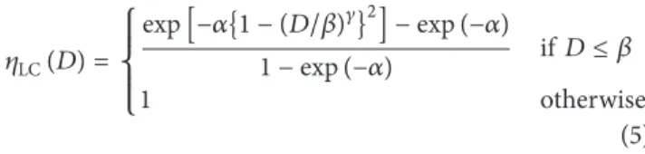
To obtain𝑤_𝑖in step 4 and (4), a weight function𝜂(⋅) that is positive and monotonically increasing is employed. In the current study, two common weight functions are tested: the one proposed by Lin and Chen [22] and the simple linear weight function (see [16]). The weight function of Lin and Chen [22] is given by 𝜂LC(𝐷) = { { { { { exp[−𝛼{1 − (𝐷/𝛽)𝛾}2] − exp (−𝛼) 1 − exp (−𝛼) if𝐷 ≤ 𝛽 1 otherwise (5) with coefficients𝛼, 𝛽, and 𝛾, where 𝛼 defines the support of the weight function and𝛽 represents the slope of decay to zero. If𝛾 = 1, then it is equivalent to the weight function of Zuo et al. [28]. The simple linear weight function mentioned in Chebana and Ouarda [16] is expressed as

𝜂CO(𝐷) = { { { { { { { 0 if𝐷 < 𝜆₁ 𝐷 − 𝜆₁ 𝜆₂− 𝜆₁ if𝜆1≤ 𝐷 ≤ 𝜆2 1 if𝐷 > 𝜆₂, (6)

where𝜆₁and𝜆₂are the coefficients with0 ≤ 𝜆₁≤ 𝜆₂≤ 1. A trial-and-error approach was applied in the current study for the parameter estimation of the weight functions. The above two weight functions𝜂LCand𝜂COare illustrated in

Figure1using strategically selected coefficients to show their roles. Figure1reveals that the weight function𝜂LCdecays to

zero quickly with high values of𝛼 (solid line with triangle). Extremely high values of𝛽 (solid line) lead this function to jump from zero to one. An extremely high value of𝛽 was used

(4)

9 8 7 6 5 4 3 2 20 19 18 17₁₆ 15 14 131 12 11 10

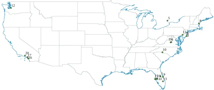
Figure 2: Locations of the retrieved stations of stormwater quality.

Table 1: Selected 20 stations list employed in Figures2and3.

Station Latitude (Decimal) Longitute (Decimal) Site Name

1 28.54 −81.37 Greenwood Urban Wetland

2 39.69 −74.25 Stafford NJ Subdiv. Colony Lakes EMCON

3 39.69 −74.26 Stafford NJ Subdivision Colony Lakes OCB

4 38.02 −78.55 29 South Buffer Strip

5 43.88 −79.46 Heritage Estates Stormwater Manag. Pond

6 39.69 −74.25 Stafford NJ Sub. Colony Lakes Soil Save

7 28.54 −81.37 Lake Olive VVRS

8 43.14 −70.86 University of New Hampshire A1

9 28.39 −80.71 FL Blvd Detention Pond

10 35.23 −80.84 Hal Marshall Bioretention Cell

11 40.04 −75.35 Villanova Traffic Island

12 47.33 −122.24 WA Ecology Embankment at SR 167 MP 16.4

13 27.17 −80.69 Lake O Sediment Demo

14 27.92 −82.77 Largo Regional STF

15 27.96 −82.45 Florida Aquarium Test Site

16 33.38 −117.57 San Onofre RVTS

17 33.87 −117.74 Yorba Linda RVTS

18 38.04 −78.48 Jensen Precast (UVA)—Phase I

19 27.99 −82.37 East Lake Outfall

20 34.28 −118.40 I-210/Filmore Street

in Chebana and Ouarda [16] and other studies. Furthermore, it is evident that𝜆₁and𝜆₂are the lower and upper limits in 𝜂CO(see the dotted line with circles in Figure1) beyond which

the weights 0 and 1, respectively, are assigned.

3. Application

The stormwater quality datasets were obtained from the international stormwater best management practice (BMP) database (http://www.bmpdatabase.org/), which has been assembled since 1996 by the American society of civil

engineers and the USEPA, as shown in Figure 2. The database was established to foster a better understanding of factors influencing urban stormwater quality; see [3,5]. The stormwater quality data as the event mean concentration of total suspended solids (TSS) was retrieved with 𝑛 ≈ 800 (see (4)), as shown in Table1, because it contains a relatively large number of records (approximately 800). The latitude and longitude were also retrieved as the GI.

As mentioned in the introduction, the KNNR is a simple model based on the conditional distribution𝑓(𝑥 | y). In Towler et al. [4], the annual average of wastewater influent concentration, longitude, and latitude were used for the

(5)

conditional variables y_𝑐 to simulate the corresponding monthly wastewater influent concentration variables. The stormwater quality data used in the present study, however, is rarely available for a continuous full year. Therefore, we use the immediate preceding monthly TSS value as the conditional variable y_𝑐 instead of the annual average as in Towler et al. [4]. In other words, the conditional variable y_𝑐 to simulate the stormwater quality for a certain month 𝜏, denoted as 𝑥_𝜏, is the stormwater quality of the preceding month (i.e., y_𝑐 = 𝑥_𝜏−1). Subsequently, Y_DBin (3) consists of all the stormwater TSS data in month𝜏 − 1. In the current study, the TSS value of the current month is simulated from the proposed DNR model by treating the GI with the depth function.

Among other coefficient sets,𝜂LCwith [𝛼 = 2, 𝛽 = 3, and

𝛾 = 0.8] and 𝜂COwith [𝜆1 = 0.1 and 𝜆2 = 0.9] performed

comparably well in the application of the current study. Therefore, the results using these coefficient sets for each weight function are presented. The models and parameter sets used in this application are:

(1) the KNNR model with the depth function (𝐷𝑀in (2))

and the weight function𝜂LCin (5) with [𝛼 = 2, 𝛽 = 3,

and𝛾 = 0.8]: DNR_LC;

(2) the KNNR model with the depth function (𝐷_𝑀) and the weight function𝜂CO in (6) with [𝜆1 = 0.1 and

𝜆₂= 0.9]: DNR_CO.

Each TSS value is simulated 500 times with the three models above. Their performances are evaluated through the mean absolute log error (MALE) and the root mean square log error (RMSLE), given, respectively, as:

MALE=∑ 𝑁𝐺 𝑡=1󵄨󵄨󵄨󵄨_{󵄨log (𝑥) − log (𝑥}𝐺𝑡)󵄨󵄨󵄨󵄨󵄨 𝑁𝐺 (7) RMSLE= √∑ 𝑁𝐺 𝑡=1(log(𝑥) − log(𝑥𝐺𝑡)) 2 𝑁𝐺 , (8)

where 𝑁𝐺 is the number of simulated times (here, 𝑁𝐺 = 500 is used) and 𝑥𝐺_𝑡 is the data generated as a surrogate of the observed data𝑥 at the 𝑡th time. Note that (i) a low value of MALE or RMSLE indicates a better reproduction of the characteristics of the observed data; (ii) RMSLE is more sensitive to outliers than MALE due to the squared formulation; and (iii) the statistics in (7) and (8) are the log-scale version of the mean absolute error (MAE) and the root mean square error (RMSE), respectively, because stormwater quality data are commonly analyzed with log-scaling; see [1,4].

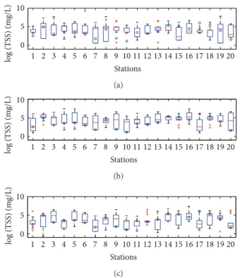
In Figure3, parts of the generated sequences (20 stations among𝑛 ≈ 800, as shown in Table1and Figure2) are illus-trated using boxplots along with the corresponding observed TSS data. The typical KNNR model often generates values that are much lower or higher than those corresponding to the observed data. The generated TSS quantities from the proposed KNNR models with depth function (DNR_CO and DNR_LC) show better agreement with the observed TSS values

1 2 3 4 5 6 7 8 9 10 11 12 13 14 15 16 17 18 19 20 0 5 10 log (T SS) (m g/L) Stations (a) 1 2 3 4 5 6 7 8 9 10 11 12 13 14 15 16 17 18 19 20 0 5 10 log (T SS) (m g/L) Stations (b) 1 2 3 4 5 6 7 8 9 10 11 12 13 14 15 16 17 18 19 20 0 5 10 log (T SS) (m g/L) Stations (c)

Figure 3: Observed value (circle) and simulated data (boxplot) of log(TSS) for (a) KNNR, (b) DNRCO, and (c) DNRLCin 20 stations as shown in Figure2. Boxes display the interquartile range (IQR) and whiskers extending to1.5×IQR. The horizontal lines inside the boxes depict the median of the data. Data beyond the whiskers (1.5 × IQR) are indicated by a plus marker (+). Note that a circle placed inside a box indicates a good agreement between the observed and simulated data.

Figure 4: Locations of all the 118 stations of stormwater quality.

than the ones from the typical KNNR model. The remaining generated values (data not shown) have a behavior similar to that described above.

To check the agreement between the observed and generated data, using all the TSS data from 118 stations, as shown in Figure 4, the MALE and RMSLE in (7) and (8) are employed. These statistics are presented in Figures 5

-6 and Table 2. The MALE statistics of the TSS-generated data at each month are illustrated in Figure5. The DNR_CO shows consistently better performance than KNNR during the summer and fall months. The DNR_LCpresents the best performance compared with the other models, except in July when DNR_CO is slightly better. The overall superiority of DNR_LCwith the average MALE metric over all the simulated

(6)

0 2 4 6 8 10 12 0.2 0.4 0.6 0.8 Month MALE KNN DNRCO DNRLC

Figure 5: Average of MALE for each month. Note that the lower value of MALE indicates better reproduction of the characteristics of all the observed TSS data shown in Figure4.

0 1 2 RMS LE KNN DNRCO DNRLC

Figure 6: Overall RMSLE for the three different nonparametric simulation models regardless of the month. Refer to Figure3.

values is briefly presented in the second row of Table1(the smallest MALE value among the three different models is illustrated).

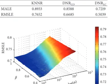
The overall simulation performance of the three models is illustrated through RMSLE, as shown in Figure 6. It shows that the RMSLEs of KNNR and DNR_CO are similar, whereas the RMSLE of DNR_LCis significantly lower than the former two. The average over all the simulated values of the RMSLE (summarized in the third row of Table1) supports the results of Figure6, indicating that the DNR_LCmodel has the lowest RMSLE, whereas KNNR and DNR_COlead to similar performances. This implies that the DNR_LCis superior to the other models.

An extensive sensitivity analysis of the coefficients for the weight function𝜂LCin (5) was performed with different

parameter sets of 𝛼 and 𝛽 while fixing 𝛾 = 2, as favored

Table 2: Overall MALE and RMSLE of the three selected nonpara-metric simulation models.

KNNR DNRCO DNRLC MALE 0.8933 0.8588 0.7219 RMSLE 0.7652 0.6685 0.5039 100 10 1 10 2 10 3 0.4 0.6 0.8 1 0.7 0.75 0.8 RMS LE 0.72 0.73 0.74 0.75 0.76 0.77 0.78 0.79 𝛽 log(𝛼)

Figure 7: Overall RMSLE with the different parameter sets [𝛼 and 𝛽] for the weight function 𝜂LC(5) after setting𝛾 = 2.

in Chebana and Ouarda [16]. This analysis is performed to further investigate the role of the coefficients of the weight function𝜂LC. The analysis of the coefficients of𝜂CO(𝜆1and

𝜆₂) is omitted because their role is obvious. The average RMSLE of each parameter set (𝛼 and 𝛽) from 500 simulations is shown in Figure7. Note that𝛼 is attributed to the shape of the weight function and 𝛽 is the location parameter beyond which the weight is assigned as the value 1.0 (see Figure1). Figure 7illustrates that(1) the RMSLE increases as𝛼 increases for all values of the parameter 𝛽 and (2) the RMSLE decreases as𝛽 increases for high values of 𝛼, whereas the decrease of RMSLE is minimal for low values of𝛼. The results indicate that𝛼 has a high impact on the performance of the model, whereas 𝛽 has little impact. Therefore, it is concluded that a low value of the parameter𝛼 and a high value of the parameter𝛽 are preferred for the currently applied TSS data.

4. Conclusion

The uncertainty in stormwater quality data has hindered the accurate analysis and physical modeling of water quality. Fitting a parametric pdf model to stormwater quality data is sometimes unfavorable primarily due to the lack of data. As an alternative, the nonparametric KNNR model was recently applied for simulating the ensemble of pollutant concentration data. In the current study, we adapted a sta-tistical approach involving “depth functions” to improve the simulation performance of the KNNR for stormwater quality data. Different weight functions are incorporated with the depth function. The results illustrate that the integration of the depth function in the KNNR model, with an appropriate choice of the weight function and its coefficients, leads to an improved performance in the simulation of stormwater

(7)

quality data. The weight function𝜂LC is superior to𝜂CO in

the simulation performance.

Automatic models for the identification of the optimal weight function and the estimation of its coefficients still remain to be developed. One feasible option to find the optimal weight function and its coefficients is to build an objective function to optimize (such as minimizing MALE and RMSLE) and then using an optimization technique such as a genetic algorithm (see [29]) or an adaptive metropolis algorithm (see [30]) to solve the optimization problem.

Conflict of Interests

The authors declare that there is no conflict of interests regarding the publication of this paper.

Acknowledgments

This work was supported by the National Research Founda-tion of Korea (NRF) Grant funded by the Korean government (MEST) (no. 2013-0362).

References

[1] US EPA, Results of the Nationwide Urban Runoff Program, Water Planning Division, Washington, DC, USA, 1983.

[2] K. M. Wong, E. W. Strecker, and M. K. Stenstrom, “Gis to estimate storm-water pollutant mass loadings,” Journal of

Environmental Engineering, vol. 123, no. 8, pp. 737–745, 1997.

[3] E. W. Strecker, M. M. Quigley, B. R. Urbonas, J. E. Jones, and J. K. Clary, “Determining urban storm water BMP effectiveness,”

Journal of Water Resources Planning and Management, vol. 127,

no. 3, pp. 144–149, 2001.

[4] E. Towler, B. Rajagopalan, C. Seidel, and R. S. Summers, “Simulating ensembles of source water quality using a K-nearest neighbor resampling approach,” Environmental Science

& Technology, vol. 43, no. 5, pp. 1407–1411, 2009.

[5] D. Park, J. C. Loftis, and L. A. Roesner, “Performance modeling of storm water best management practices with uncertainty analysis,” Journal of Hydrologic Engineering, vol. 16, no. 4, pp. 332–344, 2011.

[6] R. A. Corbit, Standard Handbook of Environmental Engineering, McGraw-Hill, New York, NY, 1989.

[7] J. W. Delleur, “The evolution of urban hydrology: past, present, and future,” Journal of Hydraulic Engineering-Asce, vol. 129, no. 8, pp. 563–573, 2003.

[8] J. Vaze and F. H. S. Chiew, “Comparative evaluation of urban storm water quality models,” Water Resources Research, vol. 39, no. 10, pp. SWC51–SWC510, 2003.

[9] J. J. Warwick and J. S. Wilson, “Estimating uncertainty of stormwater runoff computations,” Journal of Water Resources

Planning and Management, vol. 116, no. 2, pp. 187–204, 1990.

[10] R. J. Charbeneau and M. E. Barrett, “Evaluation of methods for estimating stormwater pollutant loads,” Water Environment

Research, vol. 70, no. 7, pp. 1295–1302, 1998.

[11] G. Freni, G. Mannina, and G. Viviani, “Uncertainty in urban stormwater quality modelling: the effect of acceptability thresh-old in the GLUE methodology,” Water Research, vol. 42, no. 8-9, pp. 2061–2072, 2008.

[12] U. Lall and A. Sharma, “A nearest neighbor bootstrap for resampling hydrologic time series,” Water Resources Research, vol. 32, no. 3, pp. 679–693, 1996.

[13] T. S. Lee, , Stochastic simulation of hydrologic data based on

nonparametric approaches [Ph.D. dissertation], Colorado State

University, Fort Collins, Colo, USA, 2008.

[14] T. Lee, J. D. Salas, and J. Prairie, “An enhanced nonparamet-ric streamflow disaggregation model with genetic algorithm,”

Water Resources Research, vol. 46, no. 8, Article ID W08545,

2010.

[15] J. W. Tukey, “Mathematics and the picturing of data,” in

Proceedings of the International Congress of Mathematicians, vol.

2, pp. 523–531, Vancouver, Canada, 1975.

[16] F. Chebana and T. B. M. J. Ouarda, “Depth and homogeneity in regional flood frequency analysis,” Water Resources Research, vol. 44, no. 11, Article ID W11422, 2008.

[17] R. Y. Liu, “On a notion of data depth based on random simplices,” Annals of Statistics, vol. 18, pp. 405–414, 1990. [18] R. Y. Liu and K. Singh, “A quality index based on data depth

and multivariate rank tests,” Journal of the American Statistical

Association, vol. 88, no. 421, pp. 252–260, 1993.

[19] Y. Zuo and R. Serfling, “General notions of statistical depth function,” Annals of Statistics, vol. 28, no. 2, pp. 461–482, 2000. [20] I. Mizera and C. H. M¨uller, “Location-scale depth,” Journal of

the American Statistical Association, vol. 99, no. 468, pp. 949–

966, 2004.

[21] Y. Zuo and H. Cui, “Depth weighted scatter estimators,” Annals

of Statistics, vol. 33, no. 1, pp. 381–413, 2005.

[22] L. Lin and M. Chen, “Robust estimating equation based on statistical depth,” Statistical Papers, vol. 47, no. 2, pp. 263–278, 2006.

[23] A. Caplin and B. Nalebuff, “Aggregation and social choice: a mean voter theorem,” Econometrica, vol. 59, no. 1, pp. 1–23, 1991. [24] A. K. Ghosh and P. Chaudhuri, “On maximum depth and related classifiers,” Scandinavian Journal of Statistics, vol. 32, no. 2, pp. 327–350, 2005.

[25] F. Chebana and T. B. M. J. Ouarda, “Multivariate extreme value identification using depth functions,” Environmetrics, vol. 22, no. 3, pp. 441–455, 2011.

[26] P. C. Mahalanobis, “On the generalized distance in statistics,”

Proceedings National Institute of Science of India, vol. 2, no. 1,

pp. 49–55, 1936.

[27] K. Fukunaga, Introduction to Statistical Pattern Recognition, Academic Press, San Diego, Calif, USA, 1990.

[28] Y. Zuo, H. Cui, and X. He, “On the Stahel-Donoho estimator and depth-weighted means of multivariate data,” Annals of Statistics, vol. 32, no. 1, pp. 167–188, 2004.

[29] D. E. Goldberg, Genetic Algorithms in Search, Optimization and

Machine Learning, Addison-Wesley, Reading, Mass, USA, 1989.

[30] H. Haario, E. Saksman, and J. Tamminen, “An adaptive Metropolis algorithm,” Bernoulli, vol. 7, no. 2, pp. 223–242, 2001.

(8)

Submit your manuscripts at

http://www.hindawi.com

Hindawi Publishing Corporation

http://www.hindawi.com Volume 2014

Mathematics

Journal of

Hindawi Publishing Corporation http://www.hindawi.com

Differential Equations

International Journal of

Volume 2014

Applied MathematicsJournal of

Mathematical PhysicsAdvances in

Complex Analysis

Journal of Hindawi Publishing Corporation

Optimization

Combinatorics

Function Spaces

Abstract and Applied Analysis Hindawi Publishing Corporation

http://www.hindawi.com Volume 2014 International Journal of Mathematics and Mathematical Sciences

Hindawi Publishing Corporation http://www.hindawi.com Volume 2014

The Scientific

World Journal

Discrete Dynamics in Nature and Society

Discrete Mathematics

Journal of

Evaluation of a Depth-Based Multivariate K-Nearest Neighbor Resampling Method with Stormwater Quality Data.

Research Article