Centralized dynamics multi‐frequency GNSS carrier synchronization

an author's https://oatao.univ-toulouse.fr/27096

https://doi.org/10.1109/TAES.2018.2798480

Vilà-Valls, Jordi and Closas, Pau and Fernández-Prades, Carles and Curran, James Thomas On the Mitigation of Ionospheric Scintillation in Advanced GNSS Receivers. (2018) IEEE Transactions on Aerospace and Electronic Systems, 54 (4). 1692-1708. ISSN 0018-9251

Centralized dynamics multi-frequency GNSS carrier

synchronization

Padma Bolla

Jordi Vilà-Valls

Pau Closas

Elena Simona Lohan

1_{Samara National Research University,}

Samara, Russia

2_{ISAE-SUPAERO, University of Toulouse,}

Toulouse, France

3_{Electrical and Computer Engineering}

Department, Northeastern University, Boston, Massachusetts, USA

4_{Tampere University of Technology (to}

become Tampere University from Jan 2019), Tampere, Finland

Correspondence

Padma Bolla, Samara National Research University, Samara, Russia.

Email: [email protected] Funding information

Samara National Research University, Samara, Russia; the National Science Foundation, Grant/Award Number: CNS-1815349

Abstract

In this article, we propose a new centralized multi-frequency carrier tracking architecture using an adaptive Kalman filter to enhance the loop sensitivity and reliability of individual signal tracking in challenging signal environments. The main task of the centralized dynamics-tracking filter is to effectively blend multiple frequency carrier phase observations in order to estimate the common geometric Doppler frequency of multiple-frequency received signals. Conven-tionally, multi-frequency signals are tracked independently with a fixed-loop noise bandwidth tracking approach, which is suboptimal in time-varying sig-nal environments. A suitable collaboration in multiple-frequency sigsig-nal tracking using a centralized dynamics-tracking loop enables robust carrier tracking even if some of the frequency channels are affected by ionospheric scintillation, carrier-phase multipath, or interference. Additionally, computational efficiency of the multiple-frequency tracking improves by using the proposed tracking loop architecture. Performance of the proposed multi-frequency tracking-loop architecture is verified with experiments using live multi-frequency satel-lite signals collected from GPS Block-IIF satelsatel-lites under the influence of frequency-selective interference signals.

1

I N T RO D U CT I O N

Currently, the envisaged multi-frequency Global Naviga-tion Satellite System (GNSS) signals are designed to offer several services and to meet the performance and integrity requirements of wide categories of civilian users. Each frequency signal is designed with unique signal char-acteristics, suitable for an intended civilian application and allocated to separate radio frequency (RF) spectrum in the L-band. The multiple-frequency signal transmis-sion has opened a new avenue to potential ways of using geometry-free combinations of two or more code-and carrier-phase observations, to eliminate ionosphere delay1 _{and to use in the carrier-phase integer ambiguity}

resolution.2

In a conventional multi-frequency receiver, multiple sig-nals are tracked independently by means of standard

code-and carrier-tracking loops, using delay-locked loops (DLL) and frequency/phase-locked loops (FLL/PLL), respec-tively. The pseudorange observables, which rely on the delay measurements of the code-tracking loop, are lim-ited in terms of precision by the wavelength of the code and carrier signal. Because of the independence of the tracking loops, the precision in a multi-frequency lin-ear combination of observations is limited by the lower precision of the multiple signals. In order to get mutual benefits of multiple-frequency signals and to improve the computational efficiency in signal processing, a suitable collaboration across multiple frequency signal processing can be explored, which is the motivation of the current research work.

Multiple-frequency signals transmitted from the same satellite are subject to both deterministic and nonde-terministic disturbances while propagating through the

atmosphere, causing code- and carrier-phase variations in the received signal. Some of these changes are common across multiple frequency signals, while some are spe-cific to each frequency channel. The line-of-sight (LOS) relative movement between the satellite and receiver causes signal code- and carrier-phase variations which are common across the multiple-frequency signals. Besides the common geometric phase variations, there are also channel-specific phase variations which are not common to the other channels and change the code and carrier phase in an independent manner. The inherent linear relationship between multiple-frequency signals that are synchronously generated from the same reference clock can be used to track the common-platform signal dynam-ics using a centralized tracking-loop scheme. Then, the effort to track the LOS platform dynamics with individual frequency channel PLLs can be reduced. This will enable the bandwidth of the PLL to be reduced and, thus, it will improve the noise performance in each frequency channel. The collaboration in multiple satellite signal tracking using coupled-tracking channels was initially introduced in Sennott and Senffner3_{for improved signal tracking}

per-formance in weak signal environments. The robustness of tightly coupled multi-satellite signal tracking for pre-cise positioning applications was demonstrated in Sen-nott and Senffner.4 _{Space diversity techniques such as}

coupled vector tracking loop (VTL) are well-known pro-cedures in GNSS receivers.5 _{Space diversity techniques}

enhance the individual satellite signal tracking sensitivity in weak signal environments by making use of redun-dancy of satellite signals. The VTL was introduced in Spilker6 _{for the DLL, and then the same concept was}

extended to joint carrier tracking of multi-constellation satellite signals using a vector phase-locked loop (VPLL) in.7 _{Different variants of the VTL architecture have been}

proposed by many research groups,8,9 _{and the integrity of}

VTL techniques has been an active research topic in the past decade. A VPLL for joint tracking of multiple fre-quencies and multiple satellites was presented in Henkel et al10 _{to improve the carrier-tracking loop robustness by}

mapping the tracking errors into position error, clock drift, ionospheric, and tropospheric errors. The well-known lim-itation of VTLs is the propagation of position errors in the navigation filter to all tracking channels11_{and inadequate}

update rate of the navigation filter. In the past decade, with the availability of multiple-frequency signals from the same satellite, frequency-diversity techniques, such as inter-band Doppler aiding, have been used to improve the individual signal tracking sensitivity in challenging signal environments. Recent research in Siddakatte et al12 _has

shown tracking performance improvements in fading sig-nal scenarios using combined correlator outputs based on two frequency channel tracking. Work in Vilà-Valls13

pro-posed a combined multi-frequency signal tracking using a Kalman filter (KF) to improve the tracking loop perfor-mance under ionospheric scintillation. Notice that most of the work related to multi-frequency signal tracking in the past addressed selective signal environments.

In this paper, we propose a computationally efficient and robust multi-frequency tracking architecture suitable for all signal conditions. In real GNSS signal environ-ments, multiple frequency signals from the same satel-lite often experience interference, either at the same time instant (concurrently) or at different time instants (non-concurrently). The concurrent interference is because of shadowed satellites in urban canyons and indoors, while nonconcurrent frequency selective interference is because of multipath or intentional meaconing/jamming/spoofing. To improve tracking loop performance in such chal-lenging signal environments, we propose a centralized multi-frequency signal dynamics tracking loop (CTL) architecture using an adaptive KF (AKF). The central task of the CTL is to blend multiple frequency carrier phase measurements to track common geometric Doppler shifts in the received multiple frequency signals. Additionally, a narrow bandwidth PLL is employed in each frequency channel to track the residual carrier phase variations spe-cific to each channel. The CTL AKF provides the geometric Doppler frequency estimate to individual PLLs to tune their respective carrier oscillators. Two approaches are proposed to use multiple frequency signal carrier phase measurements in order to improve tracking loop sensitiv-ity in concurrent and nonconcurrent frequency selective interference scenarios. In concurrent interference signal conditions, optimally weighted linear combinations of multiple signal phase observations are used to estimate LOS signal dynamics, while in nonconcurrent interference scenarios, stronger signal phase measurements are used. The carrier-to-noise power ratio (C∕N0)estimator in each frequency channel is used to sense the signal environment and for measurement model switching in the AKF.

A suitable collaboration in multiple frequency sig-nal tracking offers many benefits in terms of accuracy, integrity, and robustness, even if some of the frequen-cies are affected by ionosphere scintillations, multipath, or interference. The multiple frequency signal tracking using the CTL allows bandwidth reduction in individual signal carrier tracking loops by eliminating the need to track the platform dynamics. Hence, this integrated tracking loop results in precise carrier phase observations and improved dynamic performance. Additionally, the CTL provides a means to detect frequency-selective interference and an isolation scheme that can be used to verify the quality of carrier phase observations.

The paper is organized as follows. In Section 2, GNSS multi-frequency signal tracking is discussed in detail using

conventional tracking loop architecture. In Section 3, the proposed CTL architecture is introduced, and the AKF tuning methodology is detailed. Section 4 analyzes the per-formance of the new CTL. Experimental results are shown in Section 5, and finally, conclusions about the proposed CTL architecture are given in Section 6.

2

G N S S M U LT I- F R EQ U E N C Y

S I G NA L C A R R I E R T R AC K I N G

The multi-frequency GNSS signals incident on the receiver's antenna can be represented as a composite sum of individual frequency signals plus noise at the specified frequency band k, s(t) = N ∑ k=1 (√ 2PkCk(t −𝜏k)Dk(t −𝜏k)e𝑗2𝜋(𝑓Lk(t)t+𝜙k(t)) ) +nk(t), (1) where Pk is the received signal power, Ck(t) is the

pseu-dorandom code, Dk(t)is the navigation message data bits, 𝜏k is the transition delay from satellite to the receiver, 𝑓Lk(t)is the signal carrier frequency, and𝜙k(t)is the

sig-nal carrier-phase. Fisig-nally, nk(t) is the noise specific to

an individual signal frequency band. The received signal carrier phase 𝜙_k(t) represents the signal phase dynam-ics, including satellite induced Doppler, Doppler drift, and user-dynamic–induced phase variations. The received sig-nal carrier phase can be represented using Taylor's approx-imation as 𝜙k(t) =𝜙k(t0) +T . 𝜙k(t0) +T 2 2 ̈𝜙k(t0) +𝜀𝜙k, (2) where 𝜙_k(t0), .

𝜙k(t0), and ̈𝜙k(t0) are the received signal phase and its time derivatives at t0in cycles, cycles/s, and cycles/s2_{, respectively, T = t − t}

0is the signal integration time, and𝜀_𝜙k is the error in the approximation. The rate of change of phase is simply the Doppler frequency of the signal, hence, (2) can be written as

𝜙k(t) =𝜙k(t0) +T𝑓Dk(t0) + T2 2 . 𝑓Dk(t0) +𝜀𝜙k, (3) where𝑓Dk(t0), and .

𝑓Dk(t0)are the Doppler frequency and

the rate of Doppler frequency in cycles/s and cycles/s2_, respectively.

Typically, the code and carrier frequencies of multi-ple frequency signals from the same satellite are syn-chronously generated from a common reference clock. For instance, GPS L1, L2C, and L5 signals are generated synchronously from the reference clock frequency, f_ref =

10.23 MHz. Hence, the three signal code and carrier

fre-quencies are linearly related to f_refas

𝑓Lk=𝛼k𝑓re𝑓 ; 𝑓cLk =𝛽k𝑓re𝑓 ; k = {1, 2, 5}

𝛼1=154, 𝛼2=120, 𝛼5=115,

𝛽1=𝛽2=1∕10, 𝛽5 =1,

(4)

where𝑓Lkand𝑓cLkare the carrier and code frequencies of

subscripted GPS L-band signals.

The received multi-frequency GNSS signal code and carrier-phase variations are subjected to deterministic and nondeterministic disturbances due to many error sources in the propagation channel. Some of these disturbances are common across multiple frequency signals, while some are specific to each frequency channel. The common phase variations are due to LOS relative movement between the satellite and receiver. The channel-specific phase varia-tions are because of frequency-dependent error sources such as ionosphere total electron content (TEC) variations and receiver reference clock frequency drift.

The received satellite signal frequency deviation 𝑓Dk

includes the Doppler frequency due to LOS geometric shift, changes in the total electron (TEC) content of the ionosphere layer and drift in the reference clock fre-quency of the receiver with respect to the satellite clock. The geometric Doppler shift depends on the relative movement between the satellite and receiver, while the ionospheric Doppler shift depends on the signal prop-agation path through the atmosphere.14 _{The Doppler}

frequency due to reference clock frequency drift is intro-duced through a down-conversion and sampling process at the RF front-end.15_{The received satellite signal carrier}

frequency deviation at the kth frequency channel can be represented as a combination of geometric Doppler shift

𝑓GDk, and the residual Doppler shift𝑓RDk, because of

iono-spheric Doppler shift, 𝑓IDk and reference clock Doppler

shift,𝑓CDk,

𝑓Dk =𝑓GDk+𝑓RDk,

𝑓RDk =𝑓IDk+𝑓CDk.

(5) The geometric Doppler shift is significantly higher than the residual Doppler shift due to ionosphere TEC changes and drift in the reference clock frequency.

2.1

LOS - dynamics

The geometric Doppler frequency can be expressed as the velocity of the receiver relative to the transmitter in the LOS direction, scaled by the carrier wavelength. This rela-tion can be expressed as

𝑓GDk= 1 𝜆Lk (vR−vS)uLOS, 𝜆Lk𝑓GDk = (vR−vS)uLOS=𝛿 . 𝜌, (6)

where 𝜆Lk is the wavelength of the carrier signal at

satellite velocities in the LOS direction, respectively; uLOS

is the unit LOS vector from the receiver to the satellite, and

𝛿_{𝜌 is the range rate of the signal. The LOS Doppler shift is}.

in the range of ±5 kHz for a static receiver and ±10 kHz for a dynamic receiver.

From (4) and (6), the geometric Doppler shift in the code and carrier frequencies of three GPS civil signals is linearly related as

𝜆L1𝑓GDL1 =𝜆L2𝑓GDL2 =𝜆L5𝑓GDL5 (7)

𝜆c_L1𝑓cd_L1 =𝜆c_L2𝑓cd_L2 =𝜆c_L5𝑓cd_L5

where𝜆c_Lkis the wavelength of the code frequency and𝑓CDk

and𝑓GDkare the geometric Doppler shift in the code and

carrier frequency of the subscripted frequency channel. From (6), it is inferred that the LOS Doppler shift in each frequency channel is common and can be obtained from the Doppler shift or range rate of the other coexist-ing frequency signals, with appropriate scalcoexist-ing with the wavelength of the received signal carrier frequency.

2.2

Ionosphere TEC - dynamics

The changing TEC in the ionosphere layer results in an additional ionospheric Doppler shift𝑓IDk in the received

satellite signal, which is relatively small compared with the geometric Doppler shift, and can be computed as14

𝑓IDk= 1.34 × 10−7 𝑓Lk ( 𝜕(TEC) 𝜕t ) . (8)

As shown in Klobuchar,14 _{an upper limit to the rate of}

change of TEC to the stationary user is approximately 0.1×1016(el

m2∕s

)

, which results in an additional frequency shift of 0.085∕0.1∕0.1 Hz at L1/L2/L5 frequencies. From (8), we can see that the ionospheric Doppler shift is a frequency-dependent error.

2.3

Reference oscillator - dynamics

The frequency fluctuations of the main reference oscillator used to generate the reference signal in the receiver causes a Doppler shift in the down converted received signal. The reference oscillator is sensitive to the receiver platform dynamics, such as acceleration and jerk. This causes the oscillator frequency to drift over time, which will directly result in a Doppler shift in the reference signal frequency at the receiver. The drift in the reference oscillator frequency subject to the acceleration dynamics is15

Δ𝑓re𝑓 =sg𝑓re𝑓ag, (9)

where agis the acceleration in units of g (g = 9.8 m/s2), f_refis the reference clock frequency, and sgis the reference

oscillator sensitivity to the acceleration, which varies with the type of reference oscillator. Typical values of acceler-ation sensitivity are, sg = 5 × 10−9∕g for a TCXO or

sg = 3.5 × 10−9∕gfor an OCXO. The drift in the

refer-ence clock frequency corresponds to a Doppler shift in the reference carrier signal𝑓Lk, which can be expressed as

𝑓CDk=sg𝑓Lkag. (10)

For instance, at an acceleration of ag = 1g, the Doppler

shift in L1/L2/L5 reference clock frequency generation is about 7.8∕6.2∕5.8 Hz using a TCXO and 5.5∕4.2∕4.1 Hz using an OCXO. From (10), it is inferred that the influence of reference oscillator Doppler shift also depends on the received signal frequency.

The received multiple frequency signals are

down-converted to baseband using an RF front end. The down-converted signal is subsequently sampled and quantized to produce digital complex in-phase (I) and quadrature-phase (Q) signal. The digitized complex base-band data will be further processed in a digital signal processing module in three stages: acquisition, tracking, and navigation blocks. Acquisition is a onetime process that coarsely estimates the code-phase and carrier Doppler frequency of visible satellite signals. Subsequently, the code and carrier phase variations of multi-frequency signals are tracked using independent tracking loops in standard tracking loop architecture, which is discussed in the following section.

2.4

Standard multi-frequency tracking

loop architecture

A conventional frequency GNSS receiver has multi-ple individual signal code and carrier tracking channels, each one tracking a single frequency signal received from the satellite.11 _{Figure 1 illustrates the standard code and}

carrier tracking loop architecture for multiple frequency channels. The code/carrier phase tracking loop in each frequency channel is built up with a complex correlator (mixer and integrator), code/carrier phase discriminator (PD), code/carrier loop filter, and code/carrier numerically controlled oscillator (NCO). Each tracking channel syn-chronizes the receiver reference signal code and carrier frequency with that of the received satellite signal, by con-trolling the reference signal code and carrier frequency generator.

After the received signal is correlated with the local reference signal, the resultant baseband signal prompt correlator output has two components in each frequency channel k: In-Phase, IPk, and Quadrature phase, QPk,

FIGURE 1 Standard signal tracking loop for single frequency channel [Color figure can be viewed at wileyonlinelibrary.com and www.ion.org]

IPk=R(𝛿𝜏k)cos(𝜋𝛿𝑓Dk+𝛿𝜙k), (11)

QPk=R(𝛿𝜏k)sin(𝜋𝛿𝑓Dk+𝛿𝜙k),

where R(𝛿𝜏k) is the cross-correlation function between

the received and reference signal, and𝛿𝜏k,𝛿𝜙k, and𝛿𝑓Dk

are the mean code phase, carrier phase, and carrier fre-quency errors between the received and replica signals, respectively.

In the PLL carrier tracking loop, the average phase dif-ference between the received and redif-ference signals is

𝛿𝜙k(t) =𝜙k(t) − ̂𝜙k(t) (12) 𝛿𝜙k(t) =𝛿𝜙k(t0) +T𝛿𝑓Dk(t0) + T2 2 𝛿 . 𝑓Dk(t0) +𝛿𝜀𝜙k,

where𝛿𝑓Dk = 𝛿𝑓GDk +𝛿𝑓RDk is total Doppler frequency

error in each frequency channel,𝛿𝑓GDk is the geometric

Doppler frequency error, and𝛿𝑓RDk=𝛿𝑓IDk+𝛿𝑓CDkis the

residual Doppler frequency error due to ionosphere TEC variations and reference clock drift. From the complex prompt correlator outputs (IPk, QPk), the phase and

fre-quency errors in a noncoherent PLL using a two-quadrant arctangent phase discriminator can be computed as16

e_𝜙k =tan−1 ( QPk IPk ) +n_𝜙k, (13) e_𝑓k =𝛿𝜙k(t) −𝛿𝜙k(t −1) + n𝑓k,

where n_𝜙kand n_𝑓kare the phase and frequency error mea-surement noise, respectively.

The phase and frequency error measurement from the nonlinear phase discriminator output will be processed by the PLL loop filter to estimate the phase and frequency difference between the received and reference signals.

2.4.1

Design parameters of carrier

tracking loop filter

The PLL loop filter order is selected based on the expected signal dynamics. The second-order FLL-assisted third-order-PLL is preferable to bear jerking dynamics. For

a single frequency channel, an FLL-assisted PLL (F-PLL) carrier tracking loop filter can be written using an error state variable model as17

𝛿xt+1=F𝛿xt+FLzt+1, (14) where zt+1= [e𝜙k, e𝑓k] ⊤ t+1and F = ⎡ ⎢ ⎢ ⎣ 1 T T2 2 0 1 T 0 0 1 ⎤ ⎥ ⎥ ⎦ , and𝛿xt = [𝛿𝜙k, 𝛿𝑓Dk, 𝛿 . 𝑓Dk] ⊤

t are the carrier phase error,

Doppler frequency error, and Doppler rate error in cycles, cycles∕s, and cycles∕s2_{, respectively. The fixed gain matrix}

L =

[

𝛼1 𝛼2 𝛼3 0 𝛽1 𝛽2

]⊤

depends on FLL and PLL loop band-width and the coherent integration time;𝛼iand𝛽iare the

PLL and FLL filter gain coefficients, respectively.

The receiver F-PLL phase and frequency difference mea-surements have two major error sources: thermal noise error𝜎_𝜏, and steady state dynamic tracking errors,𝜙eand fe.

The F-PLL tracking loop 1-sigma threshold rule is16

𝜎𝛿𝜙=𝜎𝜏pll+

𝜙e

3 ≤ 0.26 [cycles] for the PLL (15)

𝜎𝛿𝑓 =𝜎𝜏𝑓ll+

𝑓e

3 ≤

1

12T [Hz] for the FLL

The 1-sigma values of thermal noise in the PLL and FLL can be expressed as a function of carrier tracking loop bandwidths, Bpll and Bfll, loop update interval, T,

and carrier-to noise ratio, C∕N0 (= 100.1C∕N0 for C∕N₀ in

dB-Hz), 𝜎𝜏pll= ( ₁ 2𝜋 ) √ √ √ √ √Bpll ( 1 + 1 2TC∕N0 ) C∕N0 [cycles] (16) 𝜎𝜏𝑓ll = ( ₁ 2𝜋T ) √ √ √ √ √4B𝑓ll ( 1 + 1 TC∕N0 ) C∕N0 [Hz]

The 1-sigma values of the steady state dynamic tracking bias error for the second order PLL and FLL are

𝜙e= (𝛿 ̈𝜙) w2 L =0.2809𝛿 . 𝑓 B2 pll [cycles] (17) 𝑓e= (𝛿...𝜙) w2_L =0.2809 𝛿 ̈𝑓 B2_𝑓ll [Hz]

where𝛿𝑓 and 𝛿 ̈. 𝑓 are the maximum LOS acceleration and jerk dynamics in cycles/s2_{and cycles/s}3_{, respectively; w}

Lis

the natural frequency of F-PLL, wL= 0.53 Bpll∕0.53 Bfllfor

the second order filters; and Bpll and Bfll are the loop

bandwidth of the PLL and FLL tracking loops, respectively. The carrier phase and frequency errors are functions of the tracking loop bandwidths, Bplland Bfll, integration

time, T, received signal strength, C∕N0, and signal

dynam-ics, 𝛿𝑓 and 𝛿 ̈. 𝑓. The received signal conditions cannot

be controlled, hence, the equivalent noise bandwidth in the PLL and FLL has to be chosen to accommodate the expected signal dynamics for a given C∕N0 level and sig-nal integration time. The optimal tracking loop bandwidth conditioned on the minimization of tracking loop phase and frequency error can be obtained by differentiating𝜎_𝛿𝜙 and𝜎_𝛿fwith respect to loop bandwidth and equating it to zero, ie, 𝜕𝜎𝛿𝜙

𝜕Bpll

= 0 and 𝜕𝜎𝛿𝑓

𝜕B𝑓ll = 0. This yields the following

optimal bandwidth expression for the PLL and FLL,

Bpll= ⎛ ⎜ ⎜ ⎜ ⎝ (2.35𝛿𝑓). 2 1 C∕N0 ( 1 + 1 2TC∕N0 ) ⎞ ⎟ ⎟ ⎟ ⎠ 1∕5 , (18) B_𝑓ll= ⎛ ⎜ ⎜ ⎜ ⎝ (2.35𝛿 ̈𝑓)2 4 C∕N0 ( 1 + 1 2TC∕N0 ) ⎞ ⎟ ⎟ ⎟ ⎠ 1∕5 .

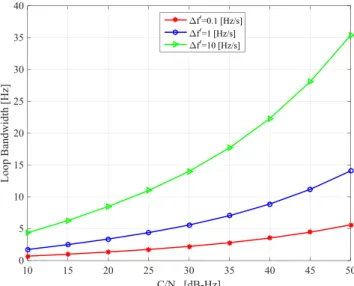
Analytical values of the optimal PLL tracking loop band-width for varying signal power levels, signal dynamics, and integration time T = 20 ms are shown in Figure 2.

A narrow loop bandwidth is beneficial at low C∕N0 lev-els to improve tracking loop noise performance at low signal dynamics, while the wide loop bandwidth is suit-able to track high signal dynamics. Finally, the objective of the tracking loop design criteria is to select the lowest bandwidth that is required to accommodate the expected signal dynamics and to meet the tracking loop error crite-ria. Hence, for efficient tracking loop operation, the noise bandwidth should be adapted to the received signal C∕N0 value and the changing signal dynamics in real time. For this reason, an adaptive scheme is needed to effectively change the equivalent noise bandwidth with respect to the signal C∕N0 value and signal dynamics estimated using the signal carrier phase error measurements. There are many approaches to realize an adaptive tracking loop with

FIGURE 2 Optimal phase-locked loops (PLL) loop bandwidth for varying C∕N0and signal dynamics [Color figure can be viewed

at wileyonlinelibrary.com and www.ion.org]

respect to changing signal environment as discussed in Vilà-Valls et al.18

It is to be noted that the C∕N0 tracking threshold for three GPS civil signals varies based on the individual signal characteristics and RF channel effects. The GPS L5 signal, with high received power and a pilot track-ing channel, has a high signal tracktrack-ing sensitivity with low C∕N0tracking threshold requirement. A suitable col-laboration in multiple frequency signal tracking loops improves the individual signal tracking sensitivity, robust-ness, and computational efficiency. However, in conven-tional multi-frequency tracking loop architectures, the inherent linear relationship between multiple frequency signals that are synchronously generated from the same reference clock in the satellite is neglected. By consider-ing the optimal trackconsider-ing loop design criteria and to address some of the limitations in conventional multi-frequency tracking loop architectures, we propose a collaborative multiple-frequency signal tracking using a CTL architec-ture, as discussed in the following section.

3

C E N T R A L I Z E D

M U LT I- F R EQ U E N C Y DY NA M I C S

T R AC K I N G LO O P A RC H I T EC T U R E

The idea of the CTL is based on the fact that the high fre-quency component of Doppler shift in the received satellite signal frequency due to LOS platform dynamics is com-mon across multiple frequency signals received from the same satellite. This common signal dynamics information can be estimated by means of a centralized dynamic track-ing filter. Thus, efforts to track them with an individual

frequency channel PLL can be reduced. This will enable the PLL bandwidth to be reduced, and thus improve the noise performance in each frequency channel. Hence, a CTL filter can be employed to track common carrier phase variations and also to improve the computational effi-ciency in multiple frequency signal tracking. Additionally, each frequency channel needs a narrow bandwidth PLL to track the residual phase variations due to frequency depen-dent error sources, such as ionosphere TEC changes and reference clock drift, as discussed earlier. An appropriate loop bandwidth to use in the PLL of each frequency chan-nel can be obtained from a prior estimation of the residual phase error.

The CTL needs to be initialized by the standard carrier tracking loop (STL), which was described in the previous section. Once all the PLLs in the STL are in phase lock, the CTL starts its operation. Figure 3 illustrates the CTL architecture, which considers a set of closed-loop narrow bandwidth PLLs and a common signal dynamics tracking loop filter. The code phase in multiple frequency channels is tracked by employing independent PLL assisted DLLs.

The CTL computes the common LOS signal dynamics information using a weighted linear combination of carrier phase and frequency error measurements from multiple frequency channels in a coordinated manner. The sum of the LOS geometric Doppler frequency information pro-vided by the CTL and the residual phase and frequency errors tracked by each frequency channel will be used to tune the carrier NCO in each channel,

𝛿 ̂𝜙k=̂zk+𝛿 ̂𝑓GDk [Hz] (19)

̂zk=𝛿 ̂𝜙0+𝛿 ̂𝑓RDk [Hz]

where𝛿 ̂𝜙k is the total control input to carrier oscillator, ̂zkis the estimate of filtered residual phase and frequency

error due to frequency dependent error sources in

sub-FIGURE 3 Centralized multi-frequency carrier tracking loop architecture [Color figure can be viewed at wileyonlinelibrary.com and www.ion.org]

scripted frequency channel, and 𝛿 ̂𝑓GDk is the geometric

Doppler shift in frequency provided by the CTL.

By the law of noise variance propagation, the noise in the control input to the carrier NCO can be expressed as

𝜎2 𝛿 ̂𝜙k =𝜎2_̂z k+𝜎 2 𝛿 ̂𝑓_GDk (20)

From (20), it is inferred that there is an extra noise induced from the CTL. The extra noise, 𝜎2

𝛿 ̂𝑓GD

, induced from the CTL has both systemic and random error compo-nents, and is correlated across multiple frequency signal tracking loop phase observations. The correlated observa-tion errors in multiple frequency channels tend to can-cel in linear combinations of pseudorange observations, such as ionosphere free and wide-lane.19_{The centralized}

dynamics tracking filter can be realized using a conven-tional higher order fixed bandwidth loop filter. However, for efficient tracking loop operation in time-varying signal environments, the noise bandwidth needs to be adapted to the received signal C∕N0 values and the changing sig-nal dynamics in real time. The AKF is considered as the most suitable solution to adapt to the changing signal environment,20_{which is discussed in the following section.}

3.1

Centralized signal dynamics tracking

via AKF

The KF is chosen to effectively blend multiple frequency channel carrier phase observations and to track com-mon LOS signal dynamics of the received multiple fre-quency signals. The signal tracking KF is regarded as identical to the DPLL with time-varying noise band-widths that optimally enhance the receiver tracking per-formance in response to user signal environments.17,21

Several state-space formulations to design a KF-based sig-nal tracking exist, depending on the measurement vari-ables and the state to be estimated. The measurement vector in the carrier tracking loop can be defined in two ways. In the first approach, the complex correlator output can be directly used as a measurement. In this case, the relationship between measurements and parameters to be estimated is nonlinear and can be solved via an extended KF (EKF). An alternative approach is to use phase dis-criminator outputs as measurements, which is adopted in the current research work, to make use of the con-ventional tracking loop measurements. The limitation of this approach is that the measurement noise is no longer an additive white Gaussian noise (AWGN). The nonlinear phase discriminator function causes the loss of the AWGN properties if the phase error crosses the linear range of the phase discriminator.

In the proposed multi-frequency signal dynamics track-ing loop architecture, the KF is replactrack-ing the FLL-assisted

PLL loop filter in conventional architectures in order to estimate the LOS carrier phase error variations in received multiple frequency signals, based on the multiple-frequency signal phase and frequency error mea-surements.

The linear state dynamic model for the error-state KF can be written as

𝛿xt+1=F𝛿xt+ Γwt, (21)

where𝛿xt is the n × 1 error-state vector at epoch t, F is

the n × n nonsingular state transition matrix from epoch

tto t + 1,𝜞 is the n × 1 noise gain vector, and wiis the

zero mean additive white Gaussian process noise sequence with variance𝜎2

wt.

The state dynamic model in the centralized

multi-frequency signal dynamics tracking KF is assumed to be a discrete Wiener process acceleration model22

to bear jerk dynamics, where the states are the carrier phase error, frequency error, and frequency rate error. The error-state dynamic model can be transformed to the trange domain by scaling with the wavelength as

[ 𝛿𝜙k 𝛿𝑓Dk 𝛿𝑓.Dk ] t+1 𝜆k= ⎡ ⎢ ⎢ ⎣ 1 T T2 2 0 1 T 0 0 1 ⎤ ⎥ ⎥ ⎦ [ 𝛿𝜙k 𝛿𝑓Dk 𝛿𝑓.Dk ] t 𝜆k+ ⎡ ⎢ ⎢ ⎣ T2 2 T 1 ⎤ ⎥ ⎥ ⎦ wt𝜆k, (22) The KF error-state vector can be written in the range domain as [ 𝛿𝜌 𝛿𝜌. 𝛿 ̈𝜌 ] t+1 = ⎡ ⎢ ⎢ ⎣ 1 T T2 2 0 1 T 0 0 1 ⎤ ⎥ ⎥ ⎦ [ 𝛿𝜌 𝛿𝜌. 𝛿 ̈𝜌 ] t + ⎡ ⎢ ⎢ ⎣ T2 2 T 1 ⎤ ⎥ ⎥ ⎦ wt𝜆k, (23)

In this model, the white noise process wt represents the

acceleration increment over the sampling period. The covariance of the process noise multiplied by the gain, 𝜞 wt, is Qt= Γ𝜎w2tΓ ⊤ ₌ ⎡ ⎢ ⎢ ⎢ ⎣ T4 4 T3 2 T2 2 T3 2 T 2 _T T2 2 T 1 ⎤ ⎥ ⎥ ⎥ ⎦ qt𝜆2_k (24)

where qt = 𝜎w2tis the process noise acceleration variance

in (cycles2_/s4_{). For this model, the practical range of𝜎}

wt

should be of the order of maximum phase acceleration increment over the sampling period.

The measurement dynamic model related to the error state vector can be represented as

zt=H𝛿xt+nt, (25)

where ztis the m × 1 measurement vector at epoch t, H

is the m × n measurement design matrix, and ntis zero

mean Gaussian measurement noise sequence with covari-ance, Rt. The single frequency channel carrier phase and

frequency measurements related to the error-state vector in the range domain can be written as

[ 𝜆ke𝜙k 𝜆ke𝑓k ] t = [ 1 0 0 0 1 0 ] [ 𝛿𝜌 𝛿𝜌. 𝛿 ̈𝜌 ] t + [ n_𝜙k n_𝑓k ] 𝜆k.

For single frequency channel tracking, Rtis a 2 × 2 matrix.

Qtand Rtare positive definite matrices (ie, Q≻ 0, R ≻ 0).

The KF requires an initialization of the state vector,𝛿x0, and state error covariance P0, and an exact knowledge of the process noise covariance Qt and measurement noise

covariance Rt, based on the prior information of the

sys-tem and signal operating environment. The steady-state KF gain can be computed as23

Kt+1=Pt+1|tHT(HPt+1|tHT+Rt+1)−1, (26)

Pt+1|t=FPt|tFT+Qt, (27)

where Kt+ 1is the 3 × 2 Kalman gain matrix at epoch t + 1. The error-state KF equations can be written as

𝛿 ̂xt+1|t =F𝛿 ̂xt|t, (28)

𝛿 ̂xt+1|t+1=𝛿 ̂xt+1|t+Kt+1̃zt+1, (29)

̃zt+1=zt+1−H𝛿 ̂xt+1|t, (30)

with̃zt+1the innovation of the measurement vector, which is used to update the predicted state vector, 𝛿 ̂xt+1|t, and

Pt+ 1|tis the prediction error covariance matrix.

The multiple-frequency signal dynamic tracking KF state-vector can be initialized with a prior estimate of phase and frequency errors, which are estimated within the STL, as 𝛿 ̂x0= [ 𝛿𝜌 𝛿𝜌. 𝛿 ̈𝜌 ] = [ 𝛿𝜙k 𝛿𝑓Dk 𝛿𝑓.Dk ] 𝜆k. (31)

The KF error-state estimate 𝛿 ̂Xt+1 is conditioned on knowing the true values of the system parameters

F, P, H, Q_tand Rt. The time-varying KF gain value is

ini-tially influenced by the initial conditions, but eventually ignores them, paying much attention to the process noise and measurement noise covariance matrices. Even then, the assumed noise statistics Qtand Rtare not

uncondition-ally valid for GNSS signal tracking in time-varying signal environments such as ionosphere scintillation, blockage and interference. Hence, in the signal tracking KF, the process noise and measurement errors must be estimated from the measurements. This process leads to tuning the KF using statistical estimation of Q_tand Rtvalues based

on the measurements.24,25_{The AKF is a suitable method}

for dynamically adjusting the parameters of the KF. There are many approaches for tuning the AKF as summarized in.26 _{An innovation-based adaptive estimation is used as}

the most suitable technique in multiple sensor fusion applications24,25_{and is used in this paper for common}

sig-nal dynamics tracking based on the multiple frequency signal carrier phase error measurements. The idea of an

innovation-based AKF is to regularly estimate measure-ment and process noise covariances using instant carrier phase error measurements. An approach to processing multi-frequency channel measurements using AKF in a time-varying GNSS signal environment is discussed in the following section.

3.2

Multi-frequency channel

measurement processing

In real GNSS signal environments, multiple frequency sig-nals are subject to either concurrent or non-concurrent fre-quency selective interference. To track the signal dynamics in such interference signal scenarios, carrier phase and frequency error measurements from multiple frequency channels can be processed in two different ways within the centralized carrier dynamics tracking KF. Namely, 1. Concurrent frequency selective interference occurs in

urban canyons and foliage, where the satellite will be shadowed for a short duration, causing all frequency signals to be attenuated or blocked at the same time. In this case, it is beneficial to combine multiple frequency channel measurements in an optimal way to obtain a minimum mean square error (MMSE) estimate of the common geometric Doppler frequency error between the received and reference signals. This approach will reduce the influence of interference in each frequency channel measurement by means of a KF gain distribu-tion. The measurement vector in this case can be rep-resented as a vector of measurements from N multiple frequency channels,

z = [z1, … , zN], (32)

This approach has limitations for use in nonconcur-rent interference scenarios, due to the propagation of errors from weak signal tracking loops to strong signal tracking loops.

2. Nonconcurrent frequency selective interference is most likely due to intentional or unintentional RF interfer-ence such as multipath, jamming, and spoofing. In such signal conditions, it is beneficial to use measure-ments from a signal frequency channel that is not under the influence of interference. This approach avoids the propagation of errors from weak signal tracking channels to stronger signal tracking channels. In a non-concurrent interference signal scenario, the mea-surement vector is chosen from multiple frequency channels based on a maximum carrier-to-noise ratio criteria,

z = max

C∕N0

[z1, … , zN]. (33)

Notice that this approach is not a suitable solution when all the frequency channels are under the influ-ence of interferinflu-ence.

The two signal conditions discussed above will be sensed by using a C∕N0 estimator in each frequency channel, compared to a C∕N0 threshold. In the former case, the optimal value KF gain weighting each frequency chan-nel measurement is computed based on the measurement noise variance. While in the latter case, signal phase and frequency error measurements from the high C∕N0 sig-nal channel will be chosen to estimate the KF error-state vector. To avoid the propagation of errors from weak sig-nal channel measurements to stronger channel measure-ments, it is necessary to sense and exclude the weak signal channel measurements from the measurement vector. The channel condition is indicated by the C∕N0 estimator to measurement switching block, in order to switch between concurrent and non-concurrent measurement models as shown in Figure 4.

In a time-varying signal environment, a reliable estima-tion of C∕N0 level of each channel is necessary to enable the dynamic operation of CTL. In general, the C∕N0 esti-mation in weak signal environments is biased from the truth. An unbiased estimate of the C∕N0 level in weak signal environments can be obtained by increasing the coherent integration time as shown in Groves.27 _More

detailed information on the C∕N0 estimation techniques in GNSS receiver can found in Groves27_{and Muthuraman}

and Borio.28_{The estimated C∕N}

0level in each channel is compared with the C∕N0threshold in order to switch the measurement models in CTL. The criteria to fix the C∕N0 threshold in CTL can be obtained through simulations and the C∕N0 tracking threshold performance of multi-ple frequency signals in standard carrier tracking loop architecture.

The carrier phase and frequency error measurements from multiple frequency channels in the phase domain will be transformed to the range domain to estimate range and range error rate using the KF. The KF error-state vec-tor which includes range error, range error rate, and range acceleration error needs to be transformed back to the

FIGURE 4 Line-of-sight (LOS) Doppler frequency estimation using an Adaptive Kalman Filter scheme [Color figure can be viewed at wileyonlinelibrary.com and www.ion.org]

phase domain by appropriate scaling with the inverse of the signal wavelength, to obtain the corresponding geo-metric Doppler frequency in each frequency channel, and then be used to tune the corresponding carrier NCO,

𝛿𝑓GDk = ( 1 𝜆k ) 𝛿_𝜌. (34)

The estimation process of measurement and process noise covariances in AKF using instant carrier phase error measurements is discussed in the following section.

3.3

Estimation of measurement

and process noise covariances

The essential step in the innovation-based AKF is the esti-mation of the innovation covariance. The covariance of the innovation sequence can be estimated using a simple moving average filter as given in Jazwinski,20

̂C̃zt = 1 M t ∑ 𝑗=t−M+1 ̃z𝑗̃zT_𝑗 (35)

wherẽztis the measurement innovation sequence, and M

is the number of samples in the window. The innovation covariance can be estimated from the measurement noise covariance as

̂C_̃zt =[HPt|t−1HT+Rt

]

(36)

In strong signal conditions, the measurement noise vari-ance in a GNSS receiver can be obtained from the C∕N0 estimator in each frequency channel carrier tracking loop, as given in Ward et al16_by 𝜎2 e_𝜙k = ( 1 4𝜋2_(C∕N 0)kT) ) ( 1 + 1 2𝜋(C∕N0)kT ) [c𝑦cles2] (37) 𝜎2 e_𝑓k = 2𝜎2 e_𝜙k T2 [( c𝑦cles2∕sec2)] (38)

While in degraded signal propagation scenarios, an alter-native way to estimate the measurement variance is using a covariance matching approach. From the KF linear mea-surement model given in (24), the meamea-surement noise at epoch t can be obtained as

̃zt =zt−H𝛿 ̂xt|t−1 (39)

By using M noise samples, the unbiased estimator of the measurement covariance R can be obtained as29

̂Rt= 1 M −1 t ∑ 𝑗=t−M+1 (( ̃z𝑗− ̂n) (̃z𝑗− ̂n)T−M −_M 1𝛄t ) (40) 𝛄t=HPt|t−1HT (41)

In the case of time-varying measurement noise covari-ance, a recursive estimation of Rt from Lr measurement

samples can be implemented as

̂nt= ̂nt−1+ 1 Lr ( ̃zt−̃zt−Lr ) (42) ̂Rt = ̂Rt−1+ 1 Lr ( (̃zt− ̂nt) (̃zt− ̂nt)T −(̃zt−Lr− ̂nt ) ( ̃zt−Lr− ̂nt )T) + 1 Lr (( ̃zt−̃zt−Lr ) ( ̃zt−̃zt−Lr )T) +Lr−1 Lr ( 𝛄t−Lr−𝛄t ) . (43)

The measurement noise covariance matrix for N inde-pendent multiple frequency channel carrier phase and frequency error measurements can be represented as a diagonal matrix, ̂Rt = diag(𝜎e2_𝜙1, 𝜎e2_𝑓1, … , 𝜎e2_𝜙N, 𝜎e2_𝑓N).

Simi-larly, the signal dynamics information which is the process noise covariance Q_t can be obtained using Doppler fre-quency rate measurements𝑓.Dkin each frequency channel.

A simple phase acceleration process noise variance estima-tion using a moving average estimator within a specified window is,30 qt= 1 M −1 t ∑ 𝑗=t−M+1 [ . 𝑓Dk(𝑗) − 1 M t ∑ 𝑗=t−M+1 [ . 𝑓Dk(𝑗) ]]2 (44) where the units of q_tare cycles2_/s4_and𝑓.

Dk(𝑗) represents

the signal phase acceleration or frequency rate measure-ment in cycles/s2 _{obtained from the difference of} con-sequent Doppler frequency outputs in the signal carrier tracking loop. The process noise covariance Qtcan be

esti-mated by substituting q_tin (24). The estimated values of Rt

and Qtcan be used to calculate the time-varying optimal

value of the KF gain in response to signal dynamics. However, the simultaneous update of Rtand Qtis not a

viable solution as they negatively affect the filter response. Hence, it is reasonable to estimate and update the mea-surement noise and process noise covariance alternatively in the Kalman gain estimation.26

3.4

Kalman filter gain adaption

to measurement error variance and signal

dynamics

In the centralized dynamics tracking loop filter, carrier phase discriminator output measurements from multi-ple frequency channels will be combined statistically in an optimal way to obtain the best possible estimate of

𝛿xt based on the time-varying estimates of Qt, Rt, and

Kt values. The process noise covariance Qt represents

the rate of change of the state, while the measurement noise covariance Rtrepresents the accuracy of the signal

measurements. The optimal weight to multiple signal car-rier phase measurements depends on individual signal measurement noise variance Rt and manifestation of the

KF gain. The Kalman gain can be represented in terms of estimated innovation covariance and Qtas

Kt= ( FPt|t−1FT+Qt ) HT̂C−1_̃z t . (45)

Then, the KF gain will be manifested based on the car-rier phase measurement noise variance and signal Doppler rate as discussed earlier. The KF equivalent noise band-width is characterized in comparison to a conventional PLL loop filter in.31,32_{The steady-state KF equivalent noise}

bandwidth can be computed from the Kalman gain, which is a function of tuning parameters Q and R as given in Won,30

Beq=

K(Q, R)

cnT

[Hz] (46)

where cnis the filter coefficient for the n-th order PLL and Tis the coherent integration time.

For a third order loop filter, cn = 3.048 and the

steady-state gain matrix K is directly proportional to Q and inversely proportional to R. This relation enables the con-struction of an adaptive filter bandwidth for time-varying signal environments. In weak signal environments, mea-surement noise variance R increases, which in turn reduces the Kalman gain. In high dynamic signal envi-ronments, the process noise increases, and as a result the Kalman gain tends to increase proportionally. The Kalman filter equivalent bandwidth changes proportionally to the gain variation in high dynamic and weak signal conditions. To evaluate the Kalman filter gain adaption in response to the changing signal power levels and dynamics, we assume that the initial values of noise statistics within the KF are P0(1, 1) = 0.52, P0(2, 2) = 1002, P0(3, 3) = 102, the process noise tuning parameter is set as q = 1 (cycles2_/s4_), the carrier phase error measurement variance𝜎2

e_𝜙1 =0.052,

and (T=0.02 s).

The time-varying optimal Kalman gain value and the equivalent noise bandwidth in the case of signal tracking KF using single frequency channel phase measurement (ie, the non-concurrent frequency selective interference case) at fixed values of Q and R is shown in Figure 5. The Kalman gain value is initially influenced by the state tran-sition covariance to measurement noise ratio, while the Kalman gain steady-state value varies in response to the process noise covariance and measurement noise covari-ance ratio. In the initial phase of filter operation, the equiv-alent noise bandwidth is wide enough to cater to the large values of carrier phase and frequency errors and is gradu-ally reduced to the steady-state fixed bandwidth value. The transient response of the Kalman filter is controlled by the process noise covariance matrix Q. The KF acts as a fixed

FIGURE 5 Discrete-time Kalman gain and equivalent noise bandwidth variation in single frequency carrier phase measurement at fixed values of noise statistics [Color figure can be viewed at wileyonlinelibrary.com and www.ion.org]

bandwidth filter in the steady-state for fixed values of Q and R.

In the case of signal dynamics tracking using a combi-nation of two frequency signal measurements (ie, the con-current frequency selective interference scenario), Kalman filter gain coefficients are adjusted to give weighting to two frequency channel measurements based on individ-ual signal measurement noise variances. For instance, we assume two frequency signal carrier phase error variances are equal,𝜎2

e_𝜙1 = 𝜎e2_𝜙2 = 0.052cycles2, hence, the Kalman

gain coefficients K(1, 1) and K(1, 2) are equal to process two frequency channel measurements with equal weight-ing. The KF equivalent noise bandwidth to each of the two frequency channel trackings is reduced to half in com-parison to single frequency channel tracking as shown in the lower panel of Figure 6. The reduced bandwidth in each frequency channel in turn reduces the requirement of the C∕N0tracking threshold and tolerance to in-band RF interference.

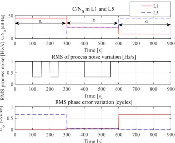
Now the KF gain adaption to the changes in signal dynamics and measurement noise variance in two fre-quency channel tracking is analyzed. The two frefre-quency signals received from the same satellite are subjected to common LOS signal dynamics, but the C∕N0level in each channel may differ depending on the influence of RF chan-nel effects. As an example, the C∕N0 level is assumed to be varying differently in two frequency channels in three regions (ie, a, b, and c) as shown in Figure 7. The common LOS signal dynamics variation in two-frequency chan-nels is represented by the process noise tuning parameter switching between q = 0.1 and 1 (cycles2_/s4_{) to represent} the low and high signal dynamics scenarios, respectively.

FIGURE 6 Discrete time Kalman gain values and equivalent noise bandwidth in two frequency channel carrier phase

measurements at fixed values of noise statistics [Color figure can be viewed at wileyonlinelibrary.com and www.ion.org]

FIGURE 7 Signal power levels and dynamics variation in received two frequency signals [Color figure can be viewed at wileyonlinelibrary.com and www.ion.org]

The KF gain coefficients are adapted proportionally to two frequency signal carrier phase error measurement statis-tics (ie, C∕N0) as shown in Figure 8. In region a, the C∕N0 level set at 45 dB-Hz in the first signal is higher than that of the second signal C∕N0 level set at 10 dB-Hz. The two frequency channel measurement noise variance is calcu-lated based on C∕N0 values and Kalman gain values are updated to offer high gain to the first frequency channel measurements in region a, while the second frequency channel measurements are excluded from the measure-ment vector as shown in Figure 8. The KF gain in the steady state is changing with respect to the signal process noise covariance, ie, q = 0.1 and 1 (cycles2_/s4_).

FIGURE 8 Discrete Kalman gain adaption in adaptive Kalman filter (AKF) to measurement noise and process noise variance of two frequency signals [Color figure can be viewed at

wileyonlinelibrary.com and www.ion.org]

In region b, the C∕N0 level in two frequency channels is reduced to 25 dB-Hz, representing the concurrent fre-quency selective interference scenario. The Kalman gain value in region b is equally distributed to process two fre-quency channel measurements. At higher signal dynam-ics, ie, q = 1 (cycles2_/s4_{), KF gain values are indeed} high even at low C∕N0values to respond to the changes in carrier frequency deviation. In region c, the first channel

C∕N0 value is significantly lower than that of the sec-ond channel. The KF gain is high for the secsec-ond signal measurements in region c and the first frequency channel measurements are excluded from the estimation process.

4

P E R FO R M A N C E A NA LY S I S O F

C E N T R A L I Z E D M U LT I- F R EQ U E N C Y

DY NA M I C S T R AC K I N G LO O P

To evaluate the performance benefits of the proposed adap-tive CTL tracking loop, a simple analysis of KF equivalent bandwidth using single and two-frequency signal mea-surements is shown with reference to standard PLL fixed loop bandwidth in Figure 9. The Kalman filter equivalent bandwidth is computed as per the relation given in (46)30

for three different signal dynamic profiles, ie, q = 0.1, 1, and 10 (cycles2_/s4_{) at a C∕N}

0of 50 dB-Hz in each frequency channel.

In CTL, either a single or combination of multiple frequency channel phase measurements is utilized to estimate the signal dynamics using AKF. In AKF, the time-varying KF gain and the equivalent bandwidth are adapted to the changing signal dynamics and to the

FIGURE 9 Comparison of Equivalent Bandwidth in fixed BW PLL Loop filter and AKF using single and two frequency channel measurements at C/N0of 50 dB-Hz [Color figure can be viewed at

wileyonlinelibrary.com and www.ion.org]

measurement noise sequentially as discussed earlier. In a frequency-selective interference scenario, where one or more frequency channels are under the influence of inter-ference, combining multiple frequency channel measure-ments causes the propagation of errors from weak signal channels to the strong signal channel tracking loop. In such a case, it is beneficial to use the relatively stronger signal channel measurements to estimate the LOS signal dynamics. In the case of the concurrent interference sce-nario, where all the frequency channels are under the influence of fading or attenuation, it is beneficial to use the optimal weighted combination of multiple frequency channel measurements to estimate LOS signal dynamics. In the concurrent interference, Kalman filter gain is dis-tributed to give appropriate weights to all the available fre-quency channel measurements based on respective signal measurement noise statistics. The equivalent noise band-width in each frequency channel tracking loop is adapted proportionally to the Kalman gain distribution across mul-tiple channel measurements. The reduced tracking loop bandwidth in each frequency channel reduces the require-ment of the C∕N0 tracking threshold. The reduced C∕N0 tracking threshold, in turn, increases the signal tracking loop tolerance to RF interference.33_{As a result, the}

influ-ence of interferinflu-ence on each frequency channel reduces proportionally to the Kalman filter bandwidth.

As an example, the 1-sigma value of carrier-phase noise in GPS L1 and L5 signal tracking loop using AKF with single and dual-frequency channel measurements is evalu-ated using analytical error models,16_{as shown in Figure 10,}

at q = 1 (cycles2_/s4_).

FIGURE 10 PLL error in L1 and L5 signal carrier tracking loop at q=1, using AKF with single and dual frequency signal phase observations in reference to fixed loop BW PLL [Color figure can be viewed at wileyonlinelibrary.com and www.ion.org]

The steady-state value of the KF equivalent bandwidth using single and dual-frequency channel measurements is 10.6 Hz and 5.7 Hz respectively at a process noise variance of q = 1 (cycles2_/s4_{), as shown in Figure 9. The single} fre-quency channel KF tracking loop has the benefit of 2 dB tracking threshold and the dual-channel KF loop has a benefit of 4 dB tracking threshold in each channel in com-parison to the 15 Hz fixed loop bandwidth PLL. In the case of the non-concurrent frequency selective interference sce-nario, where the signal dynamics are estimated using rel-atively stronger channel phase measurements and all the other frequency channels are tracked using second-order PLL of 2 Hz BW, we have a benefit of 8 dB improvement in C∕N0 tracking threshold. As a result, the narrow loop bandwidth signal tracking with LOS signal dynamics aided by CTL has reduced the C∕N0tracking threshold require-ment of 29/25 dB-Hz in STL to 21/17 dB-Hz for L1/L5 signals, respectively. This in turn increases the robust-ness to intentional and unintentional interference in each frequency channel.

The multiple frequency signals transmitted at different radio frequencies in the L-band spectrum are influenced differently by intentional and unintentional RF interfer-ence. A characterization of GPS receiver performance during RF interference34 _{and ionosphere scintillation is}

studied in.35,36 _{When the interference signal enters the}

receiver along with the intended signal, effective carrier to noise power changes34_as

(C∕N0)e𝑓𝑓 = 1 1

C∕N0

+ J∕C

QJRc

where C∕N0 is the unjammed carrier-to-noise ratio, J∕C is the jammer-to-signal carrier power ratio, QJ is a

jamming-resistance quality factor, and Rc is code rate of

the PRN code. A typical value of Q_J is 1 for single tone continuous wave (CW) interference, 1.5 for matched spec-trum (MS), and 2.2 for band-limited white noise (BLWN) spectrum.16 _{An increased value of Q}

JRc factor in (47)

results in an increased jamming resistance in the receiver. The GPS L5 and GALILEO E5 signals with 10 times higher chip rate and more received power than GPS L1 have the benefit of a higher value of the QJRcfactor, and are more

immune to RF interference than other frequency signals in GPS and GALILEO. However, when multiple frequency channels are processed by the equal receiver front end bandwidths, the influence of a broadband noise jammer is equal on all signals and increased code chipping rates do not improve the immunity.

Ionospheric scintillation is an unintentional RF interfer-ence to the GNSS receiver. Ionospheric scintillations near the poles and the equator adversely affect the operation of a receivers PLL and leads to carrier cycle slips, navigation data bit errors, and complete loss of carrier lock.37 _After

GNSS modernization, the influence of ionosphere scintil-lation at L1, L2, and L5 frequency bands is characterized by Carrano et al.38_{The GPS L1, L2, and L5 signal tracking}

performance during scintillation is assessed by analyzing the experimental data collected during the solar maximum period in.39_{These studies have concluded that the low}

car-rier frequency signals, L2C and L5 tracking is less robust to scintillation than the GPS L1 signal, despite the advanced signal characteristics such as high chip rate and power.

In light of the above discussion, the diversity in the per-formance of multi-frequency GNSS signals can be best utilized by employing the proposed CTL architecture in a GNSS receiver to complement each other in challenging signal environments such as blocking, jamming/spoofing, and ionosphere scintillation.

The performance benefits of the proposed CTL architec-ture are summarized as follows:

• Computational efficiency: The replacement of a

mul-tiple number of higher order carrier tracking loops by a single centralized dynamics tracking filter and multiple narrow bandwidth PLLs improves the computational efficiency of the GNSS receiver significantly, which in turn is a power-efficient solution.

• Restoration of temporary loss-of-lock: During the

receiver operation in a real GNSS signal environment, the signal tracking loop may lose lock for a short time interval when the frequency channel is being shadowed or blocked. In such a case, it is necessary to reacquire the signal to resume the signal tracking process after the signal reappears. The signal re-acquisition is a

computa-tionally intensive process in scalar tracking loops. In the proposed centralized dynamics multi-frequency track-ing architecture, a LOS Doppler shift aid is provided by the CTL to all the frequency channels, including the blocked channels to restore the lost tracking process after the signal reappears. This, in turn, eliminates the need for the re-acquisition process.

• Robustness to interference: In multi-frequency CTL

architecture, individual frequency signal tracking using narrow bandwidth PLL assisted by LOS Doppler fre-quency information from AKF is inherently less sen-sitive to interference than the standard tracking loop. Hence, the frequency selective interference such as jam-ming or spoofing on CTL needs higher jamjam-ming power to that of STL to disrupt the intended frequency channel tracking process.

• Robustness to spoofing: The CTL provides LOS

sig-nal dynamics aid to the narrow-band tracking loop in each frequency channel. The influence of a spoofing signal with dynamics deviated from the authentic sig-nal on selective frequency channels can be detected and rejected due to the mismatch between the received spoofing signal dynamics and authentic signal dynam-ics aided by the CTL. At most, the frequency selective spoofing impairs the targeted frequency channel from tracking the legitimate signal and leads to a jammed state. Therefore, the false signal can never be tracked by any of the spoofed channels while the authentic sig-nal dynamics are provided by the CTL. Hence, the CTL architecture improves the receiver robustness to fre-quency selective spoofing by making use of redundancy of a number of frequency signals.

• Improvement in position accuracy: The common

Doppler-aided multi-frequency channel tracking using CTL will result in common mode observation errors in multiple channels. The common-mode observation errors tend to cancel out when a linear combination of the observations are generated, such as ionosphere-free, wide-lane, etc., as shown in Bolla and Lohan.19 _This,

in turn, leads to improvement in position accuracy and precision.

5

E X P E R I M E N TA L R E S U LT S

The proposed centralized-dynamics tracking-loop archi-tecture for multiple-frequency signals is evaluated through experiments using live satellite data collected from the Block-IIF satellite constellation. A COTS (commer-cial off-the-shelf) based wide-band RF front-end SDR-Nav40 with 20.46 MHz pre-correlation bandwidth and 27.456 MHz sampling rate was used to collect L1 C/A and L5 signal data. Digitized IF data from the RF front-end was

processed in a multi-frequency software receiver, which has been tailored for this project based on.40_{The standard}

car-rier tracking loop was designed with an FLL-assisted third order PLL for multiple frequency channels with 15 Hz PLL loop filter BW and 10 Hz FLL BW. The CTL architecture was realized using one common dynamics tracking adap-tive Kalman filter and multiple narrow bandwidth second order closed loop PLLs are employed. The loop bandwidth required to track residual phase variations in each fre-quency channel was obtained from a prior estimation of residual signal phase variations through experimental data. It is to be noted that received signals with C∕N0below 30 dB-Hz are considered weak signals, while signals in the C∕N0 above 30 dB-Hz are considered stronger sig-nals based on the simulations. Hence, the measurement model switching in KF is based on the C∕N0 thresh-old of 30 dB-Hz for the experimental evaluation of CTL. The C∕N0 level in each frequency channel is estimated using a sliding window of correlation output samples and narrow-to-wideband power ratio method with an integra-tion time of one second. In strong signal condiintegra-tions, the R-matrix in the AKF is obtained from the C∕N0estimator. In weak signal conditions, the R-matrix is estimated using an alternative approach mentioned in Section 3.3. In weak signal conditions, KF gain estimation is not dependent on the C∕N0level estimation accuracy error.

From the experimental results shown in Figure 11, the residual Doppler frequency variation in each frequency channel is within the range of 2 Hz. Hence, the closed-loop PLL in each frequency channel was realized using sec-ond order PLL with 2 Hz loop bandwidth to track residual phase variations specific to each frequency channel. The centralized dynamic tracking filter was realized using a third-order adaptive Kalman filter. The initial noise statis-tics of the Kalman filter are assumed in the phase domain as P0(1, 1) = 0.52, P0(2, 2) = 1002, P0(3, 3) = 102. The pro-cess acceleration noise variance and measurement noise variance is estimated from the STL tracking loop results. The geometric Doppler variation has a slope of 1 Hz/s as shown in Figure 11, hence, a reasonable value of q = 1 (cycles2_/s4_{) and phase measurement noise variance in L1} of𝜎2e_𝜙1 =0.022(cycles2) and in L5,𝜎e2_𝜙1 =0.012(cycles2).

GNSS signals, being spread spectrum in nature, are inherently more immune to conventional jamming wave-forms such as CW, pulse signal, etc. As a result, con-ventional jamming waveforms need higher power that is beyond the thermal noise level to disrupt the receiver functionality. Moreover, with advanced receiver technol-ogy, any interference signal with power level beyond the GNSS signal dynamic range can be easily detected by an automatic gain control mechanism in the RF front and be limited before entering the signal processing stage of a receiver. Hence, an interference signal that cannot be

FIGURE 11 Geometric Doppler and residual Doppler variation of received signal in static case in L1 tracking loop using CTL [Color figure can be viewed at wileyonlinelibrary.com and www.ion.org]

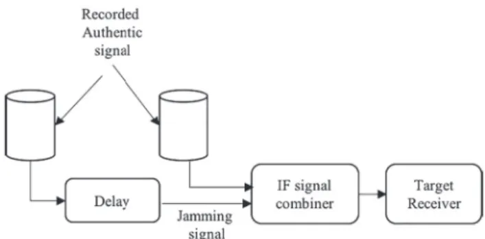
FIGURE 12 Test-set up for jamming attack

detected at the front-end and can reach out to the pro-cessing stage of a GNSS receiver is matched spectrum jamming waveform. Hence, to evaluate the performance of a proposed centralized multi-frequency dynamic tracking loop, we have considered a matched spectrum jamming waveform as a potential source. The matched spectrum jamming waveform is generated using a delayed version of the recorded signal as shown in Figure 12.

Here, we have demonstrated the performance of CTL in the cases of concurrent and non-concurrent interference in multiple frequency signals.

• Case 1: concurrent frequency selective interference:

Both L1 and L5 are jammed at J∕C of 15 dB at the same time instant.

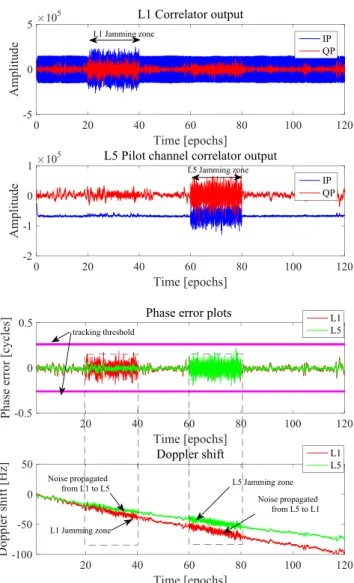
In this experiment, the LOS signal dynamics tracking using the two frequency channel measurements model in CTL is evaluated subjected to RF interference on two-frequency channels at the same time instant. As shown in Figure 13, both L1 and L5 signal channels are under the influence of matched spectrum jamming at J∕C