To link to this article : DOI :
10.1016/j.ecoinf.2017.05.006
URL :
https://doi.org/10.1016/j.ecoinf.2017.05.006
To cite this version :
Thierry, Hugo and Vialatte, Aude and Choisis,
Jean-Philippe and Gaudou, Benoit and Parry, Hazel and Monteil,
Claude Simulating spatially-explicit crop dynamics of agricultural
landscapes: The ATLAS simulator. (2017) Ecological Informatics,
vol. 40. pp. 62-80. ISSN 1574-9541
Open Archive TOULOUSE Archive Ouverte (OATAO)
OATAO is an open access repository that collects the work of Toulouse researchers and
makes it freely available over the web where possible.
This is an author-deposited version published in :
http://oatao.univ-toulouse.fr/
Eprints ID : 19064
Any correspondence concerning this service should be sent to the repository
administrator:
[email protected]
Simulating spatially-explicit crop dynamics of agricultural landscapes: The
ATLAS simulator
Hugo Thierry
a,⁎, Aude Vialatte
a, Jean-Philippe Choisis
a, Benoit Gaudou
b, Hazel Parry
c,
Claude Monteil
aaDYNAFOR, Université de Toulouse, INPT, INRA, Toulouse, France bIRIT, Université Toulouse Capitole, F-31000, Toulouse, France cCSIRO, Ecosciences Precinct, Dutton Park, 4102, Queensland, Australia
A R T I C L E I N F O
Keywords: Crop rotations Crop phenology Spatially-explicit Landscape dynamics Crop managementA B S T R A C T
The spatially-explicit AgriculTural LandscApe Simulator (ATLAS) simulates realistic spatial-temporal crop availability at the landscape scale through crop rotations and crop phenology. Intended to be linked to organism population dynamics, the simulator is developed in a multi-agent platform. The model relies on initial GIS inputs for landscape composition and configuration. Users define typical rotations and crop phenology stages to be included, according to their objectives. In the study, we present two applications to contrasting landscapes, where ATLAS is capable of simulating accurate composition (crop area) and configuration (crop clustering) dynamics. ATLAS has potential applicability to a range of contrasting agricultural landscapes. The benefits of such a simulator are the possibility to study the effects of various simulated management scenarios of crop spatial-temporal availability in relation to target organisms and/or specific ecological processes (e.g. pest, biological control), within a single model framework.
1. Introduction
Agroecosystems are characterized by high spatial and temporal in-stability, due to human management through agricultural practices such as crop rotations, and climatic conditions influencing crop phenology. Crop phenology can be defined as the timing of cyclic, climatically driven, recurring events (e.g. growth stages) of the plant. This high spatial-temporal variability of crops within agricultural landscapes has an important impact on the habitat availability for animal organisms; indeed, many depend on various resources to fulfill their life cycles (Gurr et al., 2016; Landis et al., 2000; Médiène et al., 2011). In particular, biological control of pests by natural enemies is dependent on a range of habitat availability within the agricultural landscape, and can be highly impacted by changes in the crop cover as new crops are introduced (e.g.
Vialatte et al., 2006). For example, pests such as cereal aphids will rely on different crops as nutritional resources throughout the year (Vialatte et al., 2007). Hoverflies, which are natural enemies of cereal aphids, are strongly associated with pastures and forest elements as habitats within the landscape throughout the year (Alignier et al., 2014; Sarthou et al., 2005). Thus, better comprehension of the interactions between the agricultural landscape and these populations could lead to increase in the efficiency of biological control through landscape management.
Nevertheless, studying these interactions often requires observa-tions and data gathering at large spatial and temporal scales. This can be costly and to conduct a full set of experimental studies at these scales can be challenging. Using spatially-explicit modelling can increase our knowledge on the system and allow us to explore the implications of events for which landscape-level experiments are not feasible. Many models aiming to study these interactions are based on artificial land-scapes (Bianchi et al., 2010) that can be modified at will to study dif-ferent theoretical scenarios. Realistic landscapes require mapping ef-fort, and some models include this but remain usually static through time (Parry et al., 2006). In this paper we propose an agricultural landscape model that can easily integrate with dynamic models of or-ganisms to better explore the effects of agricultural landscape dynamics on organisms.
Several models that simulate agricultural landscapes are already available. Models such as the Agricultural Production Systems sIMulator (APSIM;Holzworth et al., 2014) allow a highly detailed si-mulation of crop phenology through time, in a non-spatial context. Other agricultural landscape models such as LandSFACTS (Castellazzi et al., 2007, 2010), DYPAL (Gaucherel et al., 2006) or LUMOCAP (Van Delden et al., 2010), are on the other hand spatially-explicit and focus on agricultural practices, with the goal to explore the effects of crop
⁎Corresponding author.
allocation from year to year across the landscape to help decision-ma-kers assess potential impacts on the quality of agricultural landscapes through selected landscape indicators. These models are not intended to be linked to population dynamics and do not consider within-year crop dynamics such as sowing dates or crop phenology. Others, such as the Animal, Landscape and Man Simulation System model (Topping et al., 2003), are developed to study the interactions between organism (e.g. pest, natural enemies) population dynamics and the agricultural land-scape and thus consider crop management and phenology at a highly detailed level. All these models have an agronomical approach, with the aim of reproducing detailed agricultural practices.
Most existing models described above are defined at the farm scale. When studying ecological processes, this could lead to spatial scale mismatches which express the fact that the levels of spatial organiza-tion in landscape management and the levels of ecological funcorganiza-tioning only very rarely coincide (Pelosi et al., 2010). These mismatches con-stitute one of the main obstacles to the sustainable management of landscapes (Cumming et al., 2006). We thus identify a niche for a model reproducing realistic spatial-temporal dynamics at the landscape scale, without taking into account any social-economical level of organiza-tion. By simplifying agronomical practices we also aim at generating a model that can be applied across agricultural systems.
This paper presents the AgriculTural LandscApe Simulator (ATLAS) which is a new, open-source model available in the OpenABM platform (https://www.openabm.org/model/5416), capable of producing a realistic spatialized representation of agricultural landscapes through time with the aim of being linked to organism population dynamics. In particular, ATLAS takes into account both landscape composition and configuration, which are both known to influence population dynamics (Fahrig et al., 2011, 2015). This paper focuses on how crop elements of the landscape are handled in ATLAS. The model was developed to ex-plore a large range of scenarios through the modification of agricultural practices and landscape heterogeneity (i.e. composition and config-uration (Fahrig et al., 2011), which can lead to identifying how land-scape changes may impact on population dynamics of agriculturally beneficial and harmful organisms.
2. Methods
2.1. The ATLAS model
The AgriculTural LandscApe Simulator (ATLAS) is a spatially-ex-plicit model focusing on reproducing the general characteristic spatial-temporal patterns (composition, configuration and crop availability) of agricultural landscapes. ATLAS was developed in the GAMA modelling and simulation development environment (Grignard et al., 2013) with the following utilities. Firstly, the GAML language used in GAMA fa-cilitates object-based programming, used to describe the behavior of each field. Secondly it allows the user to readily develop agent-based simulations for organisms that link directly to ATLAS. Thirdly, GAMA easily handles GIS data through built-in functions (for example direct spatial modifications on the different elements composing a landscape in terms of shape, placement and attributes). It is also possible to export the simulated landscape and any value of the simulation parameters describing the spatial entities as shapefiles at any moment in the si-mulation. The ATLAS model is available in the OpenABMmodel library (https://www.openabm.org/model/5416). To help define input data for ATLAS, we also developed an algorithm in R (Team, 2014) detailed inSection 2.1.3.3.
Here we present the ATLAS model using part of the ODD (Overview, Design concepts, Detail) protocol for describing individual and agent-based models defined byGrimm et al. (2006, 2010).
2.1.1. Overview
2.1.1.1. Purpose. The purpose of ATLAS is to simulate a dynamic agricultural landscape reproducing the same general crop pattern
metrics as observed in the field in terms of configuration, composition and crop availability throughout the year. In the ATLAS model, landscapes are initialized using an ArcGIS shapefile, weather data and both user-defined crop rotations and phenology via a graphical user interface. The landscape is composed of patches which will each evolve individually throughout the simulation at a daily time step mainly following two processes: crops evolve through their phenology and crop fields evolve through crop rotations. It can be used to simulate a wide range of agricultural landscapes and can be interfaced with individual-based models developed for any organism that interacts with agricultural environments. This tool facilitates the spatial study of potential effects of landscape management scenarios on the interactions between landscapes and organism population dynamics. ATLAS also relies on a smaller number of parameters and inputs compared to other agricultural landscape models.
2.1.1.2. Entities, state variables, and scales. All entities, processes and variables are summarized in Fig. 1. In the ATLAS model, the environment is defined by a Landscape, composed of ‘Patch’ agents (self-contained entities which represent real world objects). A patch is a spatial entity, simply a field, a forest patch, a hedgerow or another spatial entity of the landscape, and remains fixed in dimensions and location in space and time. Each patch is assigned aLand use (e.g. Corn, Forest, Hedgerow, Other…) which defines how the patch will behave throughout the simulation, and aLand cover (e.g. CoverWheat, CoverForest, CoverBareGround) which defines what cover is actually on the patch. Each land use can either be static or dynamic through time. Any land use can be defined in ATLAS, and the level of detail (e.g. Forest or Pine Forest and Oak Forest) can be represented, depending on the needs of the scientific question to be answered. A static land use will keep the same land cover throughout the simulation with no phenology considered (e.g. forest). On the other hand, dynamic land uses evolve through time either by detailed phenological stages (i.e. crop growth throughout the season) and/or by being part of acrop rotation (which is the practice of growing a series of dissimilar/different types of crops in the same area in sequential seasons). Land covers therefore represent the current cover of the patch and are assigned certain dynamic parameters (e.g. colour, height) which are important for the visualization of the evolution of the landscape covers, but can also have a specific impact on ecological processes (e.g. potential effects of hedge height on insect movement, (Lewis, 1969; Lewis and Dibley, 1970).Crop rotations are characterized by the user with a code name and a list of the succession of crops that occur in this rotation. A ‘crop rotation’ submodel is used in ATLAS to assign the user-defined crop rotations to field patches in the landscape based on several criteria (area, clustering) detailed in theSubmodelssection. All the parameters included in ATLAS are described inAppendix A(Table A.1).
When crop patches are assigned a rotation, the land uses assigned to the patch will change over time, following the sequence defined by the rotation. The crop land use class contains all the parameters that de-termine the crop phenology. For each crop, the phenology can be chosen to be very simple (only contain info on crop sowing and harvest dates) or more detailed if there is an important relationship between the study organism and the crop phenology. For example, if the crop's stages have an impact on the population dynamics by providing re-sources to individuals (e.g. flowering crop stage in relation to pollina-tors), then the crop should be phenologically detailed if the research question is such that those dynamics should be taken into account. In this case, the crop has a specific Boolean value (“isPhenologicallyDetailed” = True) and further parameters are then needed (i.e. info on crop stages and growing degree day thresholds, see
Table A.1). Each patch growing a phenologically detailed annual crop contains a parameter that records the phenological state of the crop. Concerning detailed phenology, the current version of ATLAS only al-lows annual crops to be modeled (not perennial). Multiple crops within the year can be simulated in ATLAS.
The ‘clustered’ Land use parameter is used in the crop rotation at-tribution submodel. It is user-defined and will constrain rotation attri-bution. Rotations containing clustered crops will be assigned to patches adjacent to one another within the landscape. The clustered status of a crop (“isClustered” Boolean parameter) is defined from the data and agronomic expertise. It reflects agronomical or environmental con-straints found in the landscape (e.g. topography, distance to water) and is used to define if the crop needs to be spatially clustered or not.
Spatial scale: any scale of agricultural landscape can be taken into account (shape and size).
Temporal scale: crop rotations and phenology (described in the ODD submodels section) are driven by a record of historical climate. These climatic conditions can be considered at any hourly time step depending on data availability and to facilitate modelling sub-daily processes when organisms are added to the landscape. For example, this can be necessary when organisms have specific flight periods or diurnal/nocturnal behaviours (Kring, 1972; Shimoda and Honda, 2013). Nevertheless, landscape dynamic processes such as crop
phenology occur at a daily time step. The initial Julian day of the si-mulation and the number of simulated years can be chosen through the graphical user interface.
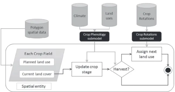
2.1.1.3. Process overview and scheduling. At a daily time step, each crop field is updated according to crop rotations and crop phenology. Other “static” elements of the landscape do not evolve through time. The different steps to achieve the update of the fields are described inFig. 2. Each crop field is assigned a land use (crop) that should be grown, defined by the crop rotation assigned to this field. Every day, the crop phenology submodel (seeSubmodelssection) evaluates if the crop is actually grown or not on the field, and if so, what phenological stage of the crop has been reached. Temperature and rain vary at a daily time step.
2.1.2. Design concepts
2.1.2.1. Basic principles. The simulation is initialized and calibrated using reference areas (mean crop area and clustering) estimated at the
landscape scale and based on a user-defined period of at least one year of data. The global pattern of the simulated landscape is intended to reflect the characteristics of the studied landscape during this period. Crop rotations should be defined in accordance with the agricultural practices observed over the same period. Because of the fact that ATLAS is driven by reference metrics estimated on a period of time, the user should be aware that exceptional events (e.g. major changes in agricultural practices such as crop introduction, or extreme climatic events such as droughts) within this period can influence the global pattern of the simulated landscape. Thus, in general we recommend focusing on periods without these events. On the other hand, ATLAS could be used as a tool with which to study the impact of such exceptional events or agricultural practices (transitions between two periods), as scenarios.
2.1.2.2. Stochasticity. Rotation assignation to each patch is partly random (see ‘assigning rotations’ submodel). In order to represent the variability farmers can face when sowing and harvesting their crops we also added stochasticity in the process (see ‘crop phenology’ submodel). 2.1.2.3. Observation. Graphical output of the model is available in 2D
and 3D, showing the spatial-temporal dynamics of the landscape (Fig. 3) using the user-defined parameters (such as name and height) for each land cover as well as the rotations simulated. All pre-defined model outputs are illustrated in Appendix B. The choice of a 3D representation of the landscape in ATLAS facilitates communication of the structure of the landscape and allows us to link land cover heights to specific population dynamics (such as movement, (Wratten et al., 2003).
2.1.3. Details
2.1.3.1. Initialization. The landscape is initialized through the input of an ESRI GIS shapefile of the landscape for any given year with available land use data. Potential crop fields are identified in the model using the land use assigned in the shapefile. Each crop field is assigned a crop rotation and a random starting point within this rotation following a deterministic uniform law (see ‘assigning rotations’ submodel). Because of the difficulty of knowing the exact phenological stage of the crops at the initial simulation date, crops that are already assigned to be growing when the model is initialized follow the non-detailed phenology model (see ‘crop phenology’ submodel). Thus, ATLAS simulations start with a burn-in period for phenologically detailed
Fig. 2. Model flow diagram for daily updating and evaluating the land covers of each field in the landscape, with the different input data and submodels represented.
crops already grown at the initialization that lasts until all initial crops are harvested.
2.1.3.2. Input data. Examples of how data should be input in the model can be found inAppendix C.
2.1.3.3. Submodels. There are two sub-models in ATLAS: rotation attribution and crop phenology.
Rotation attribution
The user can choose between two options for rotation placement in ATLAS.
Case 1. Rotations for each specific crop patch are known.
If the user wants to assign a specific rotation to each field, the ro-tation should be defined as an attribute of the field in the GIS shapefile of the landscape. The user should also define the initial crop of each patch through the “succession index” parameter in the GIS file. ATLAS will use these parameters to initialize each crop patch in the landscape. Case 2. Rotations for each crop patch are unknown.
If the rotations of each field are not known, ATLAS will assign a rotation to each field according to user-defined rotation areas and clustering constraints defined in the following section.
Firstly, the mean area assigned to each crop in the studied landscape throughout the years of data is defined. These values are used by ATLAS as reference values, which we aim to reproduce by assigning specific areas to each rotation. The mean area assigned to each crop over the years of the simulation must be equal to the reference value as it is an essential criterion for the reproduction of the global pattern of the studied landscape.
The areas to assign to each rotation are calculated through an op-timization under constraints method detailed inAppendix E. To do so, we developed an algorithm that we implemented in the software R (Team, 2014) which uses the “Least Squares with Equalities and In-equalities” method (lsei) from the limSolve package in R. The user needs to run the script in R, using the same input files (crop rotations and the reference area of each crop). An error threshold representing the percentage of error considered satisfactory between the simulated crop areas and the reference areas can be defined.
Secondly, crop clustering is taken into account, as some crops are spatially constrained in agricultural landscapes. In ATLAS, crop clus-tering is binomial. Either the model will try to maximize the crop's clustering (If the user defined the clustering parameter as True for this crop) or either the crop will place the crop randomly (If the user defined the clustering parameter as False for this crop). Estimating if a crop
should be clustered or not can be done through the combination of a clustering indicator such as the Average Nearest Neighbor Index (ANN) (e.g. as available in ArcGIS) and agronomic knowledge on specific constraints applicable to crops (e.g. distance to water points or land-scape topography).
Finally, rotations are assigned by the model to each field in the landscape. An initial field is selected by the model for each rotation, with the criteria of having a land use contained in the crop rotation. The model then assigns each rotation (following the order defined in the crop rotation csv) to remaining fields until the area assigned corre-sponds to the user-defined rotation area with a user defined error threshold. If one of the crops is clustered in this rotation, it will assign the rotation to the nearest field from the initial patch that fulfills area conditions (the sum of all patches assigned does not exceed the area calculated + the error threshold defined). If none of the crops are clustered, random patches across the landscape are assigned. The user defined error threshold represents the error acceptable in terms of area assigned to the rotation and is expressed as a percentage. Increasing this threshold can lead to increasing the difference between the simulated crop areas and the reference values, depending on the frequency of the crop within the rotation. Including this error threshold is necessary since a stochastic attribution of fields amongst the landscape does not always assign the exact area defined as an input. The last rotation is assigned to all the remaining fields. Increasing the error threshold fa-cilitates crop clustering, allowing more assignation possibilities by widening the assignation conditions. Nevertheless, we encourage the users to use the smallest error threshold first, and increase it if not satisfied with the actual crop clustering observed.
When assigning rotations, ATLAS automatically identifies all pos-sible starting points (initial land use and land cover) amongst the ro-tation's chronology based on the user-chosen initial day of the simula-tion. For each patch where a rotation is assigned, a starting point is chosen amongst all the potential ones using a discrete uniform law (each starting point has the same probability of attribution). InFig. 4, which gives an example of four potential starting points (dashed lines) for a specific four year rotation started on September 14th, two po-tential starting points can be found for the same land use (sorghum). This occurs for land uses spanning more than a year.
Crop phenology Case 1. Non-detailed crops.
Non-detailed crops are not represented using phenological stages. The crop is simply present on the field between the (fixed) crop sowing and harvest dates.
Fig. 4. Example of the possible initialization states (dashed lines) amongst one rotation (Wheat, wheat, rapeseed, sorghum rotation) with a four year duration for a specific initial date (14th of September). Land uses indicate the actual crop to be grown on the field according to the sequence defined by the rotation and the land cover indicates the actual cover simulated on the field. Each field where this rotation is assigned will be initialized (assigned a land use and land cover) at one of the starting points randomly. In this example, four starting points amongst the rotation can be identified.
Case 2. Detailed crops.
Crops with phenology that potentially influences the studied po-pulation dynamics need to be precisely modeled and are represented through detailed phenological stages. Fig. 5 describes the different processes applied to a phenologically detailed cropfield. For each re-source crop, a sowing window is defined by the initial sowing date and a maximum sowing delay defined by the user. For each patch growing this crop, a random value drawn from a uniform distribution within this window is defined as the field sowing date. This represents the con-straints farmers can face in determining an actual sowing date (machine availability, personal schedule…). Once the field sowing date is reached, the model checks if rain has fallen on that day. If so, the sowing is delayed to the next day and so on until no rain occurs.
Once the field is sown, the model calculates the number of degree-days cumulated each day (d), taking into account base temperature of the crop:
= + −
DegreeDays T (d) T (d)
2 T
d max min base
with Tmaxand Tmin representing daily maximum and minimum
tem-peratures and Tbaserepresenting the base temperature of the crop.
When the growing degree-days threshold is reached for the next phenological stage, the crop enters this stage, starting with emergence of the crop. Any phenological stages can be defined but emergence and harvestable are the only two mandatory stages. As for the sowing date, a harvest window is defined for each crop through a maximum harvest delay value defined by the user. This also represents the constraints farmers can face when planning to harvest their crops. Each patch is assigned a field harvest delay value (days) randomly chosen between 0 and the maximum harvest delay value. When the crop becomes har-vestable, the field harvest date is defined by adding the delay value to the actual day the crop becomes harvestable. When the field harvest date is reached, the farmer will be able to harvest if no rain has fallen on the harvest day. If rain has fallen then, the harvest is delayed to the next day without rain. In case of cold years with high levels of pre-cipitation, the maximum crop harvest date triggers the harvest of the crop, irrespective of its phenological stage and weather conditions. 2.2. Biological context used to calibrate and validate ATLAS
ATLAS enables exploration of the effects of landscape dynamics on organism survival and behavior. Depending on which organisms and ecological processes are studied, the scale at which crops should be detailed in terms of phenological stages will differ. In this paper, we
model two contrasting grain farming landscapes with the intention to later link them to cereal aphid dynamics. Aphids feed on cereals such as wheat, barley, corn and sorghum, and can be influenced by different crop stages (mainly through different reproduction rates, (Kieckhefer and Gellner, 1988). To fulfill their cycles, aphid populations also de-pend on crop overlapping (mainly summer/winter crops, (Gilabert et al., 2016; Vialatte et al., 2007). Thus, we will focus here on these four crops and use their dynamics to illustrate an example of what ATLAS can achieve.
2.2.1. Description of the landscapes
The first landscape, called “Vallées et Coteaux de Gascogne” (VCG), is a 620 ha (2 × 2 km2) area located in the temperate south west of France (43°16′22″ N, 0°51′7″ E). It is characterized by a high amount of native vegetation and long crop rotations mixing arable crops with pastures for mowing and livestock grazing. The second landscape, called “Bowenville” (BWN), is a 15,000 ha area (Circle with a diameter of 14 km) located in sub-tropical Queensland, Australia (27°17′39″ S, 151°26′31″ E). It represents a much more intensive agricultural system, with very low quantities of native vegetation and very short crop ro-tations, exclusively composed of arable annual crops.
The two landscapes are contrasting in terms of shape and size.Fig. 6
shows the digitized landscapes used to initialize the model for both of the landscapes. VCG was initialized using 2011field observations and BWN was initialized using 2012 field observations. VCG reference metrics were derived from three years of observations whereas BWN only had two years of available data. The mean reference areas of each crop for both landscapes can be found in Appendix D (Table D.1). Climate data was recorded using onsite weather stations forfive years (2008–2012) for both landscapes.
The land uses used for both landscapes are detailed inAppendix D
(Table D.2). Wheat, barley, sorghum and corn are modeled as possible resources for cereal aphid populations (isPhenologicallyDetailed = -True) and thus go through detailed phenological crop stages (Appendix D, Table D.3). We limited the maximum delay in both sowing and harvesting to 15 days as we consider this 2 week period to reflect the time window within which these processes usually occur within a landscape. Growing degree-day thresholds for each crop may differ between both landscapes because of the use of different cultivars, mostly region specific. The clustering status of each crop was defined according to analysis of the data using the average nearest neighbor (ANN) index and agronomic knowledge. The ANN values indicate sor-ghum as both clustered and dispersed in the data depending on the year considered (Clustering values described in theResultssection).
Fig. 5. The different factors taken into account when simulating crop growth. Farmer constraints are represented as randomly chosen delays for sowing and harvest within a time window defined by the user. Rain influences the actual sowing and harvest dates. Crop growth is entirely driven by cumulated degree-days.
Crop rotations were defined in both landscapes through agronomic expert knowledge (Table D.2). Agronomic knowledge from experts of the VCG area allowed us to determine that sorghum is usually clustered in the VCG landscape, due to spatial (water availability) and topo-graphic constraints. Sowing and harvest dates for each crop differ a lot between the landscapes because of the different seasonality in the northern and southern hemispheres. VCG is characterized by a small number of rotations with a high number of successive covers, often integrating grazing into the rotation through temporary pastures. BWN, on the contrary, is a highly intensive landscape, composed of a high number of short rotations, mostly alternating between summer and winter crops from one year to another. The areas assigned to each ro-tation were defined using the methodology explained in the roro-tation attributions submodel.
2.2.2. Simulation planning
Each landscape is simulated 30 times on a 10 year simulation. The 10 years window was chosen since it allowed the longest crop rotation to be simulated once, and others multiple times. The agricultural practices observed within a 10 year window are usually relatively stable and this period appears appropriate according to
socio-economical and global changes. The first year of the simulation (year 0) is used to initialize the crop sequences and crop phenology submodels. The error thresholds that are used to estimate the area assigned to each rotation and that are also used when assigning rotations to the land-scape are fixed at 3%. For validation purposes, the total area and the average nearest neighbor index were calculated each year for each crop. The daily area assigned to phenological stages of each crop was also collected during the simulations to explore phenology. The mean running time for 30 simulations of 10 years was under an hour on a generic desktop computer.
3. Results
The Results section is divided into two sub-sections. Firstly, we present the validation of ATLAS to the two studied agro-ecosystems by considering the general pattern of the landscape in terms of area as-signed to each crop per year and the capacity of the modeled clustering to replicate the studied landscapes. Secondly, we consider how crop phenology evolves through time and how sowing and harvest windows, defined by user-assigned delays, can influence the periods of avail-ability of each crop through time.
Fig. 6. Digitized GIS shapefiles of both the VCG (a) and BWN (b) landscapes. The land uses represented are based on the field ob-servations of the years 2011 (VCG) and 2012 (BWN).
3.1. Simulating realistic crop compositions and configurations
In the two case study agro-ecosystems, 79% (2844 out of 3600) of the simulated areas of cover of each crop were within the range of area values observed (Figs. 7 and 8). Variability from one year to another and from one simulation to another occurred; nevertheless all mean simulated areas throughout all simulations remain within the range of values observed in the data. Only temporary pastures (VCG) and sorghum (BWN) seem to be consistently underestimated, with yearly means between 5 and 15% lower than the reference value. In the BWN landscape, the yearly area assigned to corn does not vary as corn is simulated as a monoculture, thus grown in the same place year after year.
In the BWN landscape, where all crops were parameterized as clus-tered crops, 100% of the ANN values indicated a satisfactory clustering of all these crops (Table 1; values < 2.58). In the VCG landscape, a 100% replication rate of clustering is not reproduced (Table 1). Nevertheless, four crops out of the five that should be clustered are so in over 87% of the simulated years. Temporary pastures in the VCG landscape are the only exception. Considered as a clustered crop, they are efficiently clustered in the simulated landscape in only 25% of the years. This is explained by the high amount of non-crop elements fragmenting the landscape in this area and the fact that temporary pastures are essentially represented in the last rotation that was assigned.
3.2. Effects of crop phenology and weather conditions on crop availability The time frame in which fields are sown or harvested for all crops vary from one year to another, with a window of three weeks for sowing
and up to three months for harvest (Fig. 9). In the VCG landscape, 2010 (year 2) corresponds to a specifically cold and wet year and leads to delayed crop emergence (two weeks later than the other years) and harvest of crops (up to one month later). In contrast, 2011 (year 3) was a relatively hot year, leading to earlier emergence and harvest of crops (10–30 days earlier in comparison with 2010). In the fourth and fifth years of the BWN landscape, sorghum had relatively large (from 80 to 96 days) delays until harvest compared to the other years. These years correspond to meteorological years with cooler summers. On the other hand, harvest of winter crops such as barley and wheat were delayed in the first two years because of particularly cold and rainy winters, with harvest occurring up to three months later than the other years.
Phenological availability of the different resource crops simulated in both landscapes appears highly variable from one year to another (Table 2). The harvest windows of crops are wide, with up to 109 days between the earliest observed harvest and the latest across simulations in the case of Sorghum.
Weather conditions impacted the phenological stages of crops (e.g. wheat;Fig. 10). In the BWN landscape, periods of availability of crop stages can differ by up to two months depending on temperature and rainfall conditions. The VCG landscape is more homogeneous from one year to another with periods of availability for each crop stage varying for a maximum of two weeks.
4. Discussion and conclusion
The ATLAS model is capable of accurately simulating landscape composition and configuration parameters in contrasting landscapes. In
Fig. 7. Boxplots of the yearly areas assigned to each crop cover in the VCG landscape throughout 30 simulations. The three black lines in each plot represent the minimum, maximum and mean areas of the reference areas obtained through field observation.
ATLAS, mean area assigned to each crop per year is directly derived from observed data, which is used to obtain reference values. The area to assign to each rotation is estimated using a constrained optimization method with the aim of assigning a mean area to each crop as close as possible to these reference values. Thus, in both case studies, the si-mulated mean area assigned to each crop per year is within the variance of the reference values (Figs. 7 and 8). Crop rotations, and especially the assignation of a random initial cover within the rotation to each patch, drive inter-annual and inter-simulation variability of crop areas
each year. Nevertheless, 79% of the areas simulated in ATLAS each year remain within the boundaries defined by the observed data values at the study sites.
Crop clustering is efficiently reproduced for all crops in the BWN landscape (Table 2). In the VCG landscape, temporary pastures were not sufficiently clustered, with only 25% of the simulated years re-producing a clustered pattern in the landscape. This is due to the ro-tation attribution process in ATLAS. Since an error threshold is used when assigning rotations to patches of the landscape, the last rotation
Fig. 8. Boxplots of the yearly areas assigned to each crop cover in the BWN landscape throughout 30 simulations. The three black lines in each plot represent the minimum, maximum and mean areas of the reference areas obtained through field observation.
Table 1
Summary of the Average nearest neighbor values observed in the data and simulated.
Landscape Crop Data ANN values isClustered Simulated ANN values (percentage in each category) Mean simulated ANN
2010 2011 2012 Clustered
< −2.58
Random Dispersed
> 2.58
VCG Wheat − 0.76 0.89 − 1.83 False 1% 85% 14% 0.78
Rapeseed n.a − 0.28 − 2.31 True 87% 13% 0% − 2.57
Corn − 2.75 0.38 − 4.10 True 97% 3% 0% − 3.48
Temporary pasture − 2.58 − 3.82 − 4.15 True 25% 75% 0% − 0.89
Sorghum n.a 4.42 − 2.82 True 87% 13% 0% − 2.30
Sunflower − 2.08 − 2.09 − 2.30 True 90% 10% 0% − 2.71
BWN Wheat n.a − 4.83 − 5.25 True 100% 0% 0% − 9.58
Barley n.a − 6.12 − 8.12 True 100% 0% 0% − 8.20
Sorghum n.a − 7.17 − 6.01 True 100% 0% 0% − 7.27
Corn n.a − 3.51 − 3.51 True 100% 0% 0% − 3.40
Chickpea n.a n.a − 2.72 True 100% 0% 0% − 3.99
Cotton n.a − 5.33 − 7.25 True 100% 0% 0% − 5.82
The ANN values obtained through the data are listed in the table. The isClustered parameter defines how the crop was considered in ATLAS (i.e. True = clustered). The mean simulated ANN values are the result of 30 simulation runs.
considered in the attribution process can be more or less impacted depending on the error threshold defined by the user. Therefore, the user should be aware of this, and consider firstly assigning the rotations containing the most important crops for the study when setting the order of assignation of the rotations within the landscape. Overall, our binary approach could in future developments be modified to take into account the degree of clustering observed in the real landscape mea-sured by the ANN using a more complex algorithm to assign rotations within the landscape. The next step would also be to consider not just the clustering of individual crop types, but spatial alignment between crops types in space (adjacency). This would be particularly important when studying organisms with limited dispersal capabilities and strong
habitat preferences (Kennedy and Storer, 2000). This could be done by adding rules to crop rotation placements so that rotations containing crops that are usually clustered between each other are placed nearby in the landscape. Finally, clustering could also be done according to environmental factors following a similar algorithm, for example clus-tering crops around ground specificity (e.g. soil type) or water avail-ability (e.g. irrigation).
ATLAS spatially and temporally simulates crop phenological stages which is critical when studying population dynamics of organisms that respond to and depend on specific stages, such as cereal aphids. Modelling the drivers of crop availability in space and time can allow to identify periods of temporal overlap between crops leading to
Fig. 9. Areas assigned to phenologically detailed crops (wheat, barley, corn and sorghum) during the first five years of a randomly chosen simulation for the VCG landscape (a) and the BWN landscape (b). Each year represents different climate conditions defined by the data. For the VCG landscape, the second year (2010) is a particularly cold and wet year whereas the third year (2011) was the hottest and driest. In BWN, year one and two (2009 and 2010) had particularly cold winters. Year four and five (2012 and 2008) had colder summers than usual. The five years of weather data are looped and the first year is used to initialize the dynamics, explaining why 2008 data is used at the fifth year of the simulation.
Table 2
Maximum windows and mean durations of sowing and harvest of crops amongst 30 independent simulations (10 years simulated in each simulation) within both landscapes.
Land scape
Crop Mean proportion within all fields (%)
Maximum sowing window (Julian days)
Maximum harvest window (Julian days)
Mean sowing duration (days)
Mean harvest duration (days)
Mean overlapping period with…
Wheat Barley Corn Sorghum
VCG Wheat 43% 294–319 179–205 16 17.5 \ 106 104 Corn 10% 92–110 250–284 11 13 106 \ \ 164 Sorghum 2% 93–109 253–284 6.5 7 104 \ 164 \ BWN Wheat 16% 146–161 239–329 13 21.5 140 29 31 Barley 10% 116–131 230–325 13.5 22.5 140 31 35 Corn 1% 261–277 36–145 12.5 18 29 31 186 Sorghum 53% 261–277 43–152 15 28 31 35 186
The mean proportion of the crop amongst all fields throughout the simulations is described in the table. Maximum windows represent the minimum and maximum Julian days at which sowing and harvest occurred throughout the simulations. Overlapping periods are defined by the number of days both crop are simultaneously grown.
movement and colonization of pest within the landscape (Schellhorn et al., 2015; Vialatte et al., 2007). Having this knowledge can help better comprehend how populations will behave in such a landscape. This kind of approach has applicability to many biological cases such as rodent movement (Ouin et al., 2000; Rizkalla and Swihart, 2007), deer (McShea and Schwede, 1993), pollinator dynamics (Dafni, 1992) and even epidemiology simulations such as virus-related diseases (Fabre et al., 2005). The capacity to investigate the effects of management practices on populations associated with ecosystem services is the main challenge for the transition toward a more sustainable agriculture (Gaba et al., 2014). Changes in land management practices can impact differently several ecosystem services (Balbi et al., n.d.; Bennett et al., 2009). ATLAS is a novel tool that facilitates exploration of these rela-tions and the evaluation of potential management changes and their effects on ecosystem services at the landscape scale.
Other than modifying agricultural practices, ATLAS also allows spatial manipulations of the landscape elements, being able to modify the configuration and composition of the landscape to test possible effects. Further development is currently conducted to allow users to directly make these modifications in the software interface.
A constraint to the use of ATLAS is access to the necessary data for modelling a given landscape. This is a common limitation to many models in the scientific domain. Obtaining the GIS data through field survey and digitization is time consuming, costly and can be difficult depending on the studied areas. Nevertheless, the availability of GIS and weather data has been increasing throughout the past decade, especially in Europe, with the introduction of online databases and sharing technologies (e.g. PostGIS, www.postgis.net). Several studies also aim to optimize automatic methods to extract landscape elements (Fauvel et al., 2014; Herrault et al., 2013; Sheeren et al., 2009) and
could highly reduce the time necessary to digitize spatial data. Con-cerning the agricultural practice data, crop rotations and crop phe-nology are highly linked to the studied landscape and require farmer enquiries or agronomic expert advice. Future developments of ATLAS could lead to the possibility of using other crop phenology models such as APSIM (Holzworth et al., 2014) to drive crop phenology as an input in the model. The crop rotations algorithm could also be complexified by taking into account weather data and matrix based probabilities to add decision making in which crop should be grown next. Non-crop elements of the landscape also play an important role when considering organism population dynamics (e.g.Bianchi et al., 2006; Parry et al., 2015). One of the future extensions in ATLAS is taking into account phenology of perennial landscape elements and their potential effects in terms of habitats.
Finally, ATLAS is in its early days, and future development will answer to the future needs that will come from user feedback and further applications of the model. This model is currently being linked to cereal aphid dynamics and will give a first example on the possible interactions between ATLAS and population dynamics, including an exploration of the effects of landscape management on a crop damaging insect pest. The great benefits of a simplified landscape model as ATLAS is allowing to add complexity in a step by step approach, depending on the processes that need to be modeled in relation to the population dynamics, while avoiding the black box effect.
Acknowledgements
Thanks to the land holders for their participation and the Australian Grains Research Development Corporation (GRDC) for funding (CSE00051) to collect the land use data in the Australian landscape
previous version of this manuscript that greatly helped improve clarity. We also thank Mathieu Fauvel (DYNAFOR) for his advice on the crop rotation area calculation sub-model.
Appendix A. Parameters of landscape relationships and crop phenological development in the ATLAS model
Appendix B. Pre-defined outputs of the ATLAS model
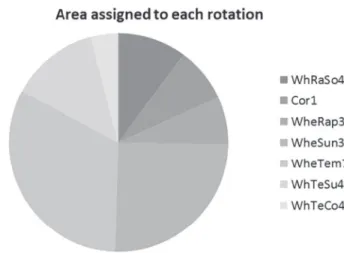
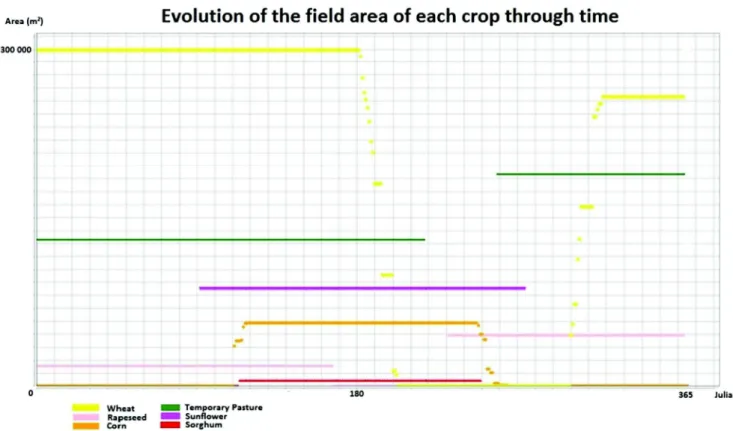
ATLAS has pre-defined outputs when simulating any agricultural landscape. The area assigned to each rotation (Fig. B.1), the current area assigned to the different crop stages of a crop (Fig. B.2) and the total areas assigned to crops through time (Fig. B.3) can be viewed in the different output tabs of the simulator. Other output statistics can be easily defined by the user according to their needs.
Table A.1
Parameters of the ATLAS model. Each patch is assigned a ‘land use’, a ‘land cover’ and when the patch is a field, a ‘crop rotation’. Example values/classes for each parameter of the model are provided.
Parameter Description Values
Landuse
name Name of the landuse Wheat, Forest, Other…
isDynamicThroughTime Defines if the landuse needs to be dynamic through time in the model, either by being part of a rotation or being phenologically detailed.
True or False
isPartOfRotation Defines if the landuse is part of a crop rotation. This defines which patches need to be assigned a rotation at the initialization of the model.
True or False
isPhenologicallyDetailed Defines if the land use should be detailed phenologically True or False isAnnual In the case of a detailed phenology, this defines which phenological submodel should be used. In the current
version of ATLAS, only annual phenology is considered.
True or False
isClustered Defined for crop landuses only. Indicates if the crop should be clustered within the landscape or not during the simulation.
True or False
Phenology related landuse parameters
startSowingDate Julian date at which sowing starts for this cover 318, 91, 257…
maximumHarvestDate Last plausible Julian date at which the cropland cover harvested 196, 274, 256… baseTemperature The base growth temperature under which the organism stops its growth. This is taken into account when
calculating the degree days.
0 °C, 6 °C…
cropSowingDelay Defines the window (in days) from the startSowingDate during which a sowing date will be chosen for the field (see crop phenology submodel)
> = 0
cropHarvestDelay Defines the window (in days) from when the crop becomes harvestable during which a harvest date will be chosen for the field (see crop phenology submodel)
> = 0
phenologicalStages A list of all the phenological stages considered for a phenologically detailed crop. Emergence, Boot, Maturity… GDDThresholds A list of the growing degree days thresholds for each phenological stage 120, 950, 1500… phenologicalHeights The height of each crop stage (meters) in the 3D representation of the landscape. > = 0 Crop rotation
name Short but meaningful name, characteristic of each rotation (for example, WhTeCo4 is a rotation of Wheat, Temporary Pasture and Corn on 4 years)
WhTeCo4
succession List of each successive crop defining the crop rotation Wheat, Wheat, Temporary pasture,
corn referenceArea Area (in any given metric) that should be assigned to the rotation in the model (see rotations attribution
submodel).
> 0
Landcover
name Name of the landcover CoverWheat,
colour Colour in rgb of the landcover in the model visualization 0:255;0:255;0:255
baseHeight Height of the land cover (in meters) in the model visualization. This height is updated depending on the crop stage for crop land covers
> = 0
Patch
rotation The crop rotation assigned to the patch (if the initial landuse is part of a rotation) WheTem7, Cor1
plannedLanduse The landuse actually assigned to the patch Wheat, Forest
currentLandcover The current landcover available on the patch CoverBareGround, CoverWheat
actualSowingDate The delay in days between the startSowingDate of the crop and the actual date of sowing From 0 to cropSowingDelay actualHarvestDate The delay in days between when the crop becomes harvestable and the actual harvest date From 0 to cropHarvestDelay
successionIndex At which stage (crop) of the rotation the patch is actually in > = 1
cropStage Stage of the current Landcover if it is a phenologically detailed crop Sowed, Boot, Flowering… GDDCumulated Number of cumulated growing degree days of the phenologically detailed crop > = 0
size Area of the patch in meters. > = 0 m
(Bowenville, Queensland). Thanks to Andrew Hulthen (CSIRO) and Jamie Hopkinson (DAFFQld) for their work ground-truthing the Australian data and advice on crop rotations respectively. Thanks to Lindsay Bell and Jeda Palmer (CSIRO) for extensive comments on a
Fig. B.2. Example of the evolution of the area assigned to each crop stage of wheat during year 1 of a VCG landscape simulation. Fig. B.1. Summary of the area assigned to each rotation within the simulated landscape.
Appendix C. Inputs needed for the ATLAS model This appendix describes the inputs needed in ATLAS. Spatial data
The user needs to input an ESRI GIS shapefile of the digitized landscape. Each patch much be assigned a land use observed from field data and the area of the polygon. An attribute may specify the rotation practiced on the field, if it is known.
Crop rotations
Typical crop rotations are user-defined in a CSV file (Table C.1). Ideally these rotations would reflect actual agricultural practices for the period simulated. The area assigned to a given rotation is calculated by the user (see ‘Crop rotations’ submodel).
Climate
ATLAS takes into account temperature and rainfall (Table C.2). ATLAS calculates the minimum, maximum and mean daily temperatures, used in the crop phenology submodel. Rain data (as a Boolean value, i.e. ‘has it rained today?’) is also necessary in relation to crop sowing and harvest (see crop phenology submodel).
If the number of years used as the input data is shorter than the number of years simulated, the model will automatically loop back to the first year of available data. The climate data files used in the model should always start at the day the simulation is initialized, which is defined by the user.
Fig. B.3. Example of the evolution of the area assigned to each crop during year 1 of a VCG landscape simulation.
Table C.1
Example of how crop rotations should be defined in the csv file used as an input of ATLAS.
Rotation Number of successive crops Area to be assigned (m2) Crop 1 Crop 2 Crop 3 Crop 4 Crop ….
CeSoCo4 4 125,758 Cereals Sorghum Cereals Corn
Cor1 1 58,410 Corn
Land uses
Each land use represented in the landscape needs to be defined in the ‘Covers’ CSV file (Table C.3). The isDynamicThroughTime parameter (true or false) defines if the land use will evolve (either as part of a rotation and/or through detailed phenology) or remain static throughout the simulation respectively. The isPartOfRotation parameter defines if this land use is part of crop rotations and if so, all patches where this land use is assigned should be assigned a rotation. The hasDetailedPhenology parameter defines the level of detail considered for this land uses phenology (see ‘Crop phenology’ submodel). The parameters startSowingDate and maximumHarvestDate define the maximum time period within which the crop is usually grown. The baseTemperature represents the base temperature (in °C) of the crop, needed to calculate the growing degree days. And finally, the isClustered parameter (explained in more detail in the crop rotations submodel) defines if this crop is usually clustered or not in the studied landscape.
Crop stages
Essential parameters include phenological stage, growing degree-day threshold associated to the stage, if the phenological stage is a potential resource for the population dynamics (e.g. interactions between the flowering stage and pollinators), and the Z height value (Table C.4). The number of phenological stages that can be simulated is user-defined. Sowing and harvest delays can also be simulated (see ‘Crop phenology’ submodel).
Land covers
Land covers are defined by a name, an abbreviation, an RGB colour and a baseHeight, which defines the height of the land cover in a 3D representation of the Landscape (Table C.5).
Table C.3
Example of the parameters characterizing each land use used in the simulation.
Name Abbreviation isDynamic ThroughTime isPartOfRotation isPhenologically Detailed isAnnual startSowingDate (Julian day) maximumHarvestDate (Julian Day) baseTemperature (°C) isClustered
Sorghum Sor True True True True 91 290 6 True
Corn Cor True True True True 91 283 6 True
Each land use is characterized by a name and an abbreviation. isDynamicThroughTime indicates if this land use will be dynamic or not through time (either through land use changes or phenology). isPartOfRotation defines if the land use is part of a crop rotation. isPhenologicallyDetailed defines if it should be phenologically detailed through crop stages. isAnnual indicates which phenology submodel should be applied, knowing only annual phenology is available in the current version of ATLAS. The isClustered parameter is used in the crop rotation attribution submodel by defining which crops should be clustered within the landscape. Finally the startSowingDate, maximumHarvestDate and baseTemperature are used in the crop phenology submodel.
Table C.2
Example of how weather data should be defined in the csv file used as an input of ATLAS. Day T °C Rain 15/09/2008 9.51 True 15/09/2008 21.22 True 15/09/2008 15.365 True 16/09/2008 9.62 True Table C.4
Example of how crop phenology of resource crops is defined in the CSV used as an input in ATLAS.
Crop Max sowing delay
Max harvest delay
Stage 1 GDD threshold 1 Resource status Stage 3D height
Stage 2 GDD threshold 2 Resource status Stage 3D height
Sorghum 15 15 Emergence 120 True 0.1 Boot 936 True 0.5
Corn 15 15 Emergence 120 True 0.1 Boot 940 True 0.5
Each crop is defined by a maximum sowing and harvest delay. Then each crop stage is characterized within the table, through a name, a growing degree-days threshold at which the crop stage is reached, a resource status and a 3D height (in meters).
Table C.5
Example of how land covers are defined in the CSV used as an input in ATLAS.
Name Abbreviation ColourR ColourG ColourB BaseHeight
CoverSorghum Sor 255 137 137 10
CoverCorn Cor 247 150 70 10
Appendix D. Initialization parameters of the ATLAS model
This appendix presents the parameter values used to initialize both landscapes in our simulations.
Table D.1
Areas (km2) assigned to each crop within each year of data and the reference value (mean of all years) used to initialize ATLAS for both landscapes.
Landscape Crop Area
2010 (km2) Area 2011 (km2) Area 2012 (km2) Reference value (km2) VCG Wheat 1.206 1.164 1.025 1.132 Rapeseed 0.024 0.101 0.246 0.126 Corn 0.221 0.265 0.268 0.251 Temporary pasture 0.809 0.777 0.671 0.752 Sorghum 0 0.056 0.138 0.064 Sunflower 0.280 0.359 0.238 0.292 BWN Wheat n.a 17.266 21.138 19.202 Barley n.a 11.061 12.913 11.987 Sorghum n.a 63.903 60.542 62.223 Corn n.a 1.116 1.116 1.116 Chickpea n.a 0 5.116 2.558 Cotton n.a 23.316 18.647 20.981 Table D.2
Description of all the land uses used to simulate both landscapes in ATLAS.
Landscape Name Code isDynamic
ThroughTime isPartOf Rotation isPhenologically Detailed IsAnnual startSowingDate (Julian day) maximumHarvest Date (Julian day)
BaseTemperature (°C)
IsClustered
VCG Sorghum Sor True True True True 91 290 6 True
Corn Cor True True True True 91 283 6 True
Rapeseed Rap True True False True 230 166 0 True
Sunflower Sun True True False True 91 274 0 True
Temporary Pasture
Tem True True False True 258 217 0 True
Wheat Whe True True True True 293 227 0 False
Fallow Fal False
Other Crop Oth False
Forest For False
South Edge SEd False North Edge NEd False Building Road Bui False
Water Wat False
Permanent Pasture
Per False
Hedge Hed False
BWN Corn Cor True True True True 260 151 6 True
Chickpea Chi True True False True 166 364 0 True
Barley Bar True True True True 115 334 0 True
Sorghum Sor True True True True 260 151 6 True
Cotton Cot True True False True 274 151 0 True
Wheat Whe True True True True 145 335 0 True
FallowSummer FaS True True False True 152 89 0 False
FallowWinter FaW True True False True 1 212 0 False
Other Crop Oth False Native
Vegetation
Nat False
Unclassified Unc False Permanent
Pasture
Per False
Water Wat False
Each land use is characterized by a name and an abbreviation code. isDynamicThroughTime indicates if this land use will be dynamic or not through time (either through land use changes or phenology). isPartOfRotation defines if the land use is part of a crop rotation. isPhenologicallyDetailed defines if the land use should be phenologically detailed through crop stages. isAnnual indicates which phenology submodel should be applied, knowing only annual phenology is available in the current version of ATLAS. The isClustered parameter is used in the crop rotation attribution submodel by defining which crops should be clustered within the landscape. Finally the startSowingDate, maximumHarvestDate and baseTemperature are used in the crop phenology submodel.
Appendix E. Method for assigning areas to each rotation in the landscape
Here we present how we calculate the area to assign to each rotation in the landscape in order to obtain realistic composition values, using an optimization algorithm.
The following notations are used throughout this appendix:
Cmax:number of possible crops Rmax:number of provided rotations
AcRef: reference area of crop c(mean of the yearly areas observed throughout the data) AcSim: simulated area of crop c
P(c | r): proportion of appearence of crop c within rotation r
P(c)Ref: proportion of crop c amongst all crops within the landscape obtained from the data P(c)Sim: proportion of crop c among all crops within the landscape simulated in ATLAS
Our aim is to calculate AcSimfor each crop as close as possible to the AcRefvalues. For the following calculations, we rewrite the areas of each crop
as proportions of the total crop allocated area (Eqs.(1) and (2)).
= ∑= P(c) A A Ref c Ref c 1 C c Ref max (1) = ∑= P(c) A A Sim c Sim c 1 C c Sim max (2) Thus, this gives us the following least squares optimization criteria (Eq.(3)):
∑
⎛ ⎝ ⎜ − ⎞ ⎠ ⎟ = min P(c) P(c) c 1 C Sim Ref 2 Max (3) P(c)Simvalues are the variables in this system and can also be expressed using Eq.(4), with P(c, r) being the joint probability of having crop c androtation r at the same time.
∑
= = P(c)Sim P(c, r) r 1 Rmax (4) Using the Bayes formula, Eq.(4)can be rewritten:Table D.3
Description of each of the crop stages considered for the four resource crops considered in the simulations.
Landscape VCG BWN
Crop Sorghum Corn Wheat Corn Barely Sorghum Wheat
Max sowing delay 15 15 15 15 15 15 15
Max harvest delay 15 15 15 15 15 15 15
Crop stage 1 Emergence Emergence Emergence Emergence Emergence Emergence Emergence
GDD threshold 120 120 80 120 120 120 80
Resource status True True True True True True True
Crop stage 2 Boot Boot Boot Boot Boot Boot Boot
GDD threshold 936 940 855 940 810 936 855
Resource status True True True True True True True
Crop stage 3 Head Head Head Head Head Head Head
GDD threshold 972 990 935 990 900 972 935
Resource status True True True True True True True
Crop stage 4 Flowering Flowering Flowering Flowering Flowering Flowering Flowering
GDD threshold 1285 1200 970 1500 940 1485 970
Resource status True True True True True True True
Crop Stage 5 Harvestable Harvestable Maturity Harvestable Maturity Harvestable Maturity
GDD Threshold 1961 1961 1670 2461 1650 2461 1670
Resource status True True True True True True True
Crop stage 6 Harvestable Harvestable Harvestable
GDD threshold 2670 2650 2170
Resource status True True True
Each crop is defined by a maximum sowing and harvest delay. Then each crop stage is characterized within the table, through a name, a cumulated growing degree day threshold and a resource status. The growing degree-day thresholds for each crop stage vary amongst one crop in both landscapes since these values are cultivar specific. The resource status indicates if the phenological stage will be of importance when linked to the studied population dynamics.
= P(c | r)P(r) P(c)Sim r 1 R =
∑
max (5) To solve the system, P(r) needs to be estimated using a method of optimization under two constraints (Eq. (6)).⎧ ⎨⎩∑ =≥ = ∈ … Constraints: r 1 P(r) 1 R P(r) 0 (for r {1, , Rmax }) max (6) The optimization method used is the “Least Squares with Equalities and Inequalities” method (lsei) from the limSolve package in R. The
simulated error for each crop (Errc) is represented as the difference between AcSim and AcRef (Eq. (7)).
Errc=im |A−cS AcRef| (7)
The user is then able to define an error threshold (ErrUser), representing the maximum Errc values that suite his needs for the simulation of the
studied landscape (Eq. (8)). ≤ c ≤
0 |Err | ErrUser (8)
If the simulated values are acceptable, the area to assign to each rotation is calculated using P(r). If no acceptable values are reached, the user should redefine the rotations containing the crops that do not manage to obtain satisfactory values.
References
Alignier, A., Raymond, L., Deconchat, M., Menozzi, P., Monteil, C., Sarthou, J.-P., Vialatte, A., Ouin, A., 2014. The effect of semi-natural habitats on aphids and their
natural enemies across spatial and temporal scales. Biol. Control 77, 76–82. Balbi, S., del Prado, A., Gallejones, P., Geevan, C.P., Pardo, G., Pérez-Miñana, E., Manrique, R., Hernandez-Santiago, C., Villa, F., n.d. Modeling trade-offs among ecosystem services in agricultural production systems. Environ. Model. Softw. doi:http://dx.doi.org/10.1016/j.envsoft.2014.12.017.
Bennett, E.M., Peterson, G.D., Gordon, L.J., 2009. Understanding relationships among multiple ecosystem services. Ecol. Lett. 12, 1394–1404.
Bianchi, F.J.J., Booij, C.J., Tscharntke, T., 2006. Sustainable pest regulation in agri-cultural landscapes: a review on landscape composition, biodiversity and natural pest control. Proc. R. Soc. B Biol. Sci. 273, 1715–1727. http://dx.doi.org/10.1098/rspb. 2006.3530.
Bianchi, F.J.J.A., Schellhorn, N.A., Buckley, Y.M., Possingham, H.P., 2010. Spatial variability in ecosystem services: Simple rules for predator‐mediated pest suppres-sion. Ecol. Appl. 20 (8), 2322–2333.
Castellazzi, M.S., Matthews, J., Wood, G.A., Burgess, P.J., Conrad, K.F., Perry, J.N., 2007. LandSFACTS: software for spatio-temporal allocation of crops to fields. In: Proceedings of 5th Annual Conference of the European Federation of IT in Agriculture, Glasgow, UK.
Castellazzi, M.S., Matthews, J., Angevin, F., Sausse, C., Wood, G.A., Burgess, P.J., Brown, I., Conrad, K.F., Perry, J.N., 2010. Simulation scenarios of spatio-temporal arrange-ment of crops at the landscape scale. Environ. Model. Softw. 25, 1881–1889. Cumming,
G., Cumming, D.H., Redman, C., 2006. Scale mismatches in social-ecological systems: causes, consequences, and solutions. Ecol. Soc. 11 (1).
Dafni, A., 1992. Pollination Ecology: A Practical Approach. IRL Press Ltd.
Fabre, F., Plantegenest, M., Mieuzet, L., Dedryver, C.A., Leterrier, J.-L., Jacquot, E., 2005. Effects of climate and land use on the occurrence of viruliferous aphids and the epidemiology of barley yellow dwarf disease. Agric. Ecosyst. Environ. 106, 49–55. http://dx.doi.org/10.1016/j.agee.2004.07.004.
Fahrig, L., Baudry, J., Brotons, L., Burel, F.G., Crist, T.O., Fuller, R.J., Sirami, C., Siriwardena, G.M., Martin, J.-L., 2011. Functional landscape heterogeneity and an-imal biodiversity in agricultural landscapes. Ecol. Lett. 14, 101–112.
Fahrig, L., Girard, J., Duro, D., Pasher, J., Smith, A., Javorek, S., King, D., Lindsay, K.F., Mitchell, S., Tischendorf, L., 2015. Farmlands with smaller crop fields have higher within-field biodiversity. Agric. Ecosyst. Environ. 200, 219–234.
Fauvel, M., Planque, C., Sheeren, D., la Mura, M.D., Cokelaer, F., Chanussov, J., Talbot, H., 2014. Robust path opening versus path opening for the detection of hedgerows in rural landscapes. In: Geoscience and Remote Sensing Symposium (IGARSS), 2014 IEEE International. IEEE, pp. 4910–4913.
Gaba, S., Lescourret, F., Boudsocq, S., Enjalbert, J., Hinsinger, P., Journet, E.-P., Navas, M.-L., Wery, J., Louarn, G., Malézieux, E., 2014. Multiple cropping systems as drivers for providing multiple ecosystem services: from concepts to design. Agron. Sustain. Dev. 1–17.
Gaucherel, C., Giboire, N., Viaud, V., Houet, T., Baudry, J., Burel, F., 2006. A domain-specific language for patchy landscape modelling: the Brittany agricultural mosaic as a case study. Ecol. Model. 194, 233–243.
Gilabert, A., Gauffre, B., Parisey, N., Le Gallic, J.-F., Lhomme, P., Bretagnolle, V., Dedryver, C.-A., Baudry, J., Plantegenest, M., 2016. Influence of the surrounding landscape on the colonization rate of cereal aphids and phytovirus transmission in autumn. J. Pest. Sci. 1–11.
Grignard, A., Taillandier, P., Gaudou, B., Vo, D.A., Huynh, N.Q., Drogoul, A., 2013. GAMA 1.6: advancing the art of complex agent-based modeling and simulation. In:
PRIMA 2013: Principles and Practice of Multi-Agent Systems. Springer, pp. 117–131. Grimm, V., Berger, U., Bastiansen, F., Eliassen, S., Ginot, V., Giske, J., Goss-Custard, J., Grand, T., Heinz, S.K., Huse, G., 2006. A standard protocol for describing individual-based and agent-individual-based models. Ecol. Model. 198, 115–126.
Grimm, V., Berger, U., DeAngelis, D.L., Polhill, J.G., Giske, J., Railsback, S.F., 2010. The ODD protocol: a review and first update. Ecol. Model. 221, 2760–2768. Gurr, G.M., Wratten, S.D., Landis, D.A., You, M., 2016. Habitat management to suppress
pest populations: progress and prospects. Annu. Rev. Entomol. 62, 91–109. Herrault, P.-A., Sheeren, D., Fauvel, M., Paegelow, M., 2013. Automatic extraction of
forests from historical maps based on unsupervised classification in the CIELab color space. In: Vandenbroucke, D., Bucher, B., Crompvoets, J. (Eds.), Geographic Information Science at the Heart of Europe, Lecture Notes in Geoinformation and Cartography. Springer International Publishing, pp. 95–112.
Holzworth, D.P., Huth, N.I., Zurcher, E.J., Herrmann, N.I., McLean, G., Chenu, K., van Oosterom, E.J., Snow, V., Murphy, C., Moore, A.D., 2014. APSIM–evolution towards a new generation of agricultural systems simulation. Environ. Model. Softw. 62, 327–350.
Kennedy, G.G., Storer, N.P., 2000. Life systems of polyphagous arthropod pests in tem-porally unstable cropping systems. Annu. Rev. Entomol. 45, 467–493. Kieckhefer, R.W., Gellner, J.L., 1988. Influence of plant growth stage on cereal aphid
reproduction. Crop Sci. 28, 688–690.
Kring, J.B., 1972. Flight behavior of aphids. Annu. Rev. Entomol. 17, 461–492. Landis, D.A., Wratten, S.D., Gurr, G.M., 2000. Habitat management to conserve natural
enemies of arthropod pests in agriculture. Annu. Rev. Entomol. 45, 175–201. Lewis, T., 1969. The distribution of flying insects near a low hedgerow. J. Appl. Ecol.
443–452.
Lewis, T., Dibley, G.C., 1970. Air movement near windbreaks and a hypothesis of the mechanism of the accumulation of airborne insects. Ann. Appl. Biol. 66, 477–484. McShea, W.J., Schwede, G., 1993. Variable acorn crops: responses of white-tailed deer
and other mast consumers. J. Mammal. 74, 999–1006.
Médiène, S., Valantin-Morison, M., Sarthou, J.-P., de Tourdonnet, S., Gosme, M., Bertrand, M., Roger-Estrade, J., Aubertot, J.-N., Rusch, A., Motisi, N., 2011. Agroecosystem management and biotic interactions: a review. Agron. Sustain. Dev. 31, 491–514.
Ouin, A., Paillat, G., Butet, A., Burel, F., 2000. Spatial dynamics of wood mouse (Apodemus sylvaticus) in an agricultural landscape under intensive use in the Mont Saint Michel Bay (France). Agric. Ecosyst. Environ. 78, 159–165.
Parry, H.R., Evans, A.J., Morgan, D., 2006. Aphid population response to agricultural landscape change: a spatially explicit, individual-based model. Ecol. Model. 199, 451–463. http://dx.doi.org/10.1016/j.ecolmodel.2006.01.006.
Parry, H.R., Eagles, D., Kriticos, D.J., Venette, R., 2015. Simulation modelling of long-distance windborne dispersal for invasion ecology. Pest Risk Model. Mapp. Invasive Alien Species 7, 49.
Pelosi, C., Goulard, M., Balent, G., 2010. The spatial scale mismatch between ecological processes and agricultural management: Do difficulties come from underlying theo-retical frameworks? Agric. Ecosyst. Environ. 139 (4), 455–462.
Rizkalla, C.E., Swihart, R.K., 2007. Explaining movement decisions of forest rodents in fragmented landscapes. Biol. Conserv. 140, 339–348.
Sarthou, J., Ouin, A., Arrignon, F., Barreau, G., Bouyjou, B., 2005. Landscape parameters explain the distribution and abundance of Episyrphus balteatus (Diptera: Syrphidae). Eur. J. Entomol. 102, 539.
Schellhorn, N.A., Gagic, V., Bommarco, R., 2015. Time will tell: resource continuity bolsters ecosystem services. Trends Ecol. Evol. 30, 524–530. Sheeren, D., Bastin, N., Ouin, A., Ladet, S., Balent, G., Lacombe, J.-P., 2009. Discriminating small wooded elements in rural landscape from aerial photography: a hybrid pixel/object-based analysis approach. Int. J. Remote Sens. 30, 4979–4990.
2003. ALMaSS, an agent-based model for animals in temperate European landscapes. Ecol. Model. 167, 65–82.
Van Delden, H., Stuczynski, T., Ciaian, P., Paracchini, M.L., Hurkens, J., Lopatka, A., Shi, Y., Prieto, O.G., Calvo, S., van Vliet, J., 2010. Integrated assessment of agricultural
policies with dynamic land use change modelling. Ecol. Model. 221, 2153–2166. Vialatte, A., Simon, J.-C., Dedryver, C.-A., Fabre, F., Plantegenest, M., 2006. Tracing individual movements of aphids reveals preferential routes of population transfers in agroecosystems. Ecol. Appl. 16, 839–844.
Vialatte, A., Plantegenest, M., Simon, J.-C., Dedryver, C.-A., 2007. Farm-scale assessment of movement patterns and colonization dynamics of the grain aphid in arable crops and hedgerows. Agric. For. Entomol. 9, 337–346.
Wratten, S.D., Bowie, M.H., Hickman, J.M., Evans, A.M., Sedcole, J.R., Tylianakis, J.M., 2003. Field boundaries as barriers to movement of hover flies (Diptera: Syrphidae) in cultivated land. Oecologia 134, 605–611.
Shimoda, M., Honda, K., 2013. Insect reactions to light and its applications to pest management. Appl. Entomol. Zool. 48, 413–421.
Team, R.C., 2014. R: A Language and Environment for Statistical Computing. R Foundation for Statistical Computing, Vienna, Austria (2012. Open Access Available Httpcran R-Proj. Org.).