1
Multivariate shift testing for hydrological variables, review,
comparison and application
F. Chebana1*
M.-A. Ben Aissia1
T. B. M. J. Ouarda1,2
1 Statistical Hydroclimatology Research Group, 490, Rue de la Couronne, Quebec, Qc,
Canada, G1K 9A9.
2 Institute Center for Water and Environment (iWATER)
Masdar Institute of Science and Technology, PO Box 54224, Abu Dhabi, UAE.
* Corresponding author: [email protected]
Abstract
1
Hydrological frequency analysis (HFA) is commonly used for the assessment of the risk 2
associated to hydrological events. HFA is generally based on the assumptions of homogeneity, 3
independence and stationarity of the hydrological data. Hydrological events are often described 4
through a number of dependent characteristics, such as peak, volume and duration for floods. 5
Unfortunately, in this multivariate setting, the verification of the above assumptions is often 6
neglected. When a shift occurs in a data series, it can affect the stationarity and the homogeneity 7
of the data. The objective of this paper is to study tests for shift detection in multivariate 8
hydrological data. The considered shift tests are mainly based on the notion of depth function, 9
except for one test that is considered for comparison purposes. A simulation study is performed to 10
evaluate and compare the power of all these tests with hydrological constraints. A flood analysis 11
application is also carried out to show the practical aspects of the considered tests. The power of 12
the considered tests is influenced by a number of factors, including the sample size, the shift 13
amplitude, the magnitude of the series and the location of the shift in the series. 14
15
Keywords:
shift, hypothesis testing, multivariate, stationarity, homogeneity, flood, depth. 161. Introduction
18
In general, in order to perform the statistical analysis of hydrological data a number of fundamental 19
assumptions are required. More precisely, preliminary testing for stationarity, homogeneity and 20
independence is a necessary step in any hydrologic frequency analysis (HFA) study [e.g. Rao and 21
Hamed, 2000]. One or more of these assumptions can fail because of a number of reasons. For 22
instance, the assumption of stationarity may not be verified because of a regime shift that can be 23
due to an abrupt change in the watershed characteristics caused by natural or anthropogenic actions 24
on the physical environment, such as deforestation or the construction of a hydraulic structure [e.g. 25
Bobée and Ashkar, 1991; Burn and Hag Elnur, 2002, Ouarda and El-Adlouni, 2011]. Because of 26
the growing evidence concerning climate change, the common assumption of stationarity of 27
hydrologic phenomena may no longer hold. The presence of shifts in data series is highlighted in 28
several hydrometeorological studies, such as floods [Seidou and Ouarda, 2007], precipitation 29
[Beaulieu et al., 2008, 2010; Ouarda et al., 2014; Chen et al., 2016], low-flows [Ehsanzadeh et al., 30
2011], wind speed [Naizghi and Ouarda, 2016], and temperature data [Jandhyala et al., 2014]. 31
The analysis of multivariate events is of particular interest in several applied fields, including 32
hydrology. Indeed, complex hydrological events, such as floods, droughts and storms are 33
multivariate events characterized by a number of correlated variables. For instance, volume (V), 34
peak (Q) and duration (D) describe floods [Ouarda et al., 2000; Shiau, 2003; Yue et al., 1999]. The 35
use of univariate HFA can lead to inaccurate estimation of the risk associated to a given event. 36
Recently, several studies adopted the multivariate framework to treat extreme hydrological events, 37
see e.g. [Chebana, 2013] for a summary and recent references. 38
HFA is composed of four main steps: i) descriptive and explanatory analysis, ii) verification of the 39
basic assumptions including stationarity, homogeneity and independence, iii) modeling and 40
estimation, and iv) risk evaluation and analysis. In the univariate setting, these steps are extensively 41
treated [e.g. Rao and Hamed, 2000]. In the multivariate context, the first two steps (i and ii) 42
attracted considerably less attention than the two others. For an overview of step i) in the 43
multivariate framework, the reader is referred to Chebana and Ouarda [2011]. Checking the basic 44
assumptions (step ii) is generally ignored in the hydrological literature in the multivariate setting. 45
For instance, it is not treated in Kao and Govindaraju [2007], Song and Singh [2009] and 46
Vandenberghe et al. [2010]. This step has a significant impact on steps iii) and iv). Therefore, 47
ignoring step ii) may lead to inaccurate models and hence to wrong results and inappropriate 48
decisions regarding resource management and infrastructure design. In order to avoid the loss of 49
human lives and property associated with design event underestimation, or the increase in 50
construction cost associated with overestimation, it is necessary to treat step ii) for a sound and 51
complete multivariate HFA. 52
Non-stationarity is a very wide notion and includes in particular the presence of one or several 53
shifts in the data. Recently, Chebana et al. [2013] provided a review and application of multivariate 54
nonparametric tests for monotonic trends and presented approaches that can be considered as a 55
preliminary step in a complete multivariate HFA. Chebana et al. [2013] indicated that, for 56
multivariate hydrological data, various types of non-stationarities can be found for which 57
appropriate tests should by reviewed, compared and applied. 58
The available literature on shift detection in the hydrological context is focused on the univariate 59
setting. Nevertheless, statistical literature exists for the general multivariate setting. Hence, existing 60
comparisons and evaluations of the proposed tests are based on scenarios and hypotheses that are 61
not adapted to the hydrological context (e.g. sample size, scale, and distributions). In addition, these 62
comparative studies are not exhaustive and are often not based on quantifiable performance criteria. 63
Consequently, there is a need for comparative studies that consider all available tests and are 64
representative of hydrological reality, scale and constraints. 65
Several multivariate shift tests are based on the concept of depth function. The latter is a statistical 66
notion to measure the depth (or its opposite, the outlyingness) of a given point with respect to a 67
multivariate data cloud or its underlying distribution. Depth functions were developed in the 68
seventies and have been receiving increasing interest [e.g. Tukey, 1975; Liu, 1990; Zuo and 69
Serfling, 2000; Mizera and Müller, 2004; Zuo and Cui, 2005; Lin and Chen, 2006; Liu and Singh, 70
2006; Chebana and Ouarda 2011; Singh and Bárdossy, 2012; Lee et al., 2014; Wazneh et al., 71
2013; 2015]. Depth functions provide a scale-standardized measure of the position of any data 72
point relative to the center of the distribution due to its affine-invariant property [Li and Liu, 2004]. 73
For the location shift, this property allows us to view the depth-based test statistics as scale-74
standardized measures. Therefore, depth-based tests can be performed without the difficulty of 75
estimating the variance of the null sampling distributions. Instead, the decision rule is derived by 76
obtaining p-values using the idea of permutation. 77
The objectives of the present paper are: 1) to show the importance of the testing step in a 78
multivariate HFA, in particular shift testing, 2) to review shift tests that are available in the 79
statistical literature and which are applicable to hydrological variables within the multivariate HFA 80
context, and 3) to perform an overall evaluation and comparison of these tests under hydrological 81
constraints (such as short sample size, specific distributions). 82
This paper is organized as follows. Section 2 introduces the definitions and notations related to the 83
shift concept. The considered tests are described in Section 3. The simulation study to evaluate the 84
performance of these tests is presented in Section 4. Section 5 illustrates an application of the 85
reviewed tests on hydrological data. The conclusions of the study and a number of perspectives are 86
reported in Section 6. 87
2. Shift concept
88
A shift can be defined by the date at which at least one feature of a statistical model (e.g., location, 89
scale, intercept and trend) undergoes an abrupt change [Seidou et al., 2007]. A large number of 90
techniques can be found in the literature to identify the date of a potential shift and to check its 91
significance. Most of the methodologies use statistical hypothesis testing to detect shifts in the 92
slope or intercept of linear regression models [Easterling and Peterson, 1995; Vincent, 1998; Lund 93
and Reeves, 2002]. For instance, Solow [1987], Easterling and Peterson [1995], Vincent [1998], 94
Lund and Reeves [2002] and Wang [2003] used the Fisher test to compare a model with and without 95
a shift. The Student and Wilcoxon tests can also be applied sequentially to detect shifts in data 96
series [Beaulieu et al., 2007, 2008]. 97
Note that not all shift approaches are based on hypothesis testing. For instance, Wong et al. [2006] 98
used the grey relational method [Moore, 1979; Deng, 1989] for single shift detection in stream flow 99
data series. In some rare cases, curve fitting methods were used [e.g. Sagarin and Micheli, 2001; 100
Bowman et al., 2006]. Extensive reviews of shift detection and correction methodologies in 101
hydrology and climate sciences can be found in Peterson et al. [1998] and Beaulieu et al. [2009]. 102
To define a shift, let
xi i1,...,n be a given d-variate dataset and 1s n be a possible shift. If such 103s exists, the series is divided into two subsamples with sizes s and m = n-s such that: 104
1 1 1 1 ,..., ,..., ,..., ,..., s s m s n y y x x z z x x (1)
105Denote by G1 and G2 respectively the cumulative distribution functions of these two subsamples. 106
The two distributions G1 and G2have the same form, except for the location, i.e. G x1( )G x2( δ) 107
for all xRd where δRdis a constant vector. Consequently, when testing the presence of a shift 108
at a position s of the series , the null and alternative hypotheses are respectively: 109
0: 0 i.e. there is no location shift
H δ
(2)
110
1: 0 i.e. there are two different subsamples at least in one component of
H δ δ
.
(3)
111
3. The considered tests
112
In the present paper, several tests to detect a shift in the location of multivariate series are 113
considered. Except for the C-test, all the presented tests are based on depth functions. The C-tests 114
is considered for comparison purposes. More details are given below regarding p-value evaluation. 115
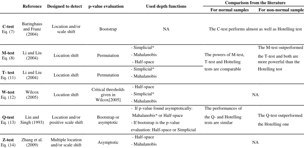
Table 1 presents a summary of the tests considered in this study. 116
3.1. Depth functions
117
The absence of a natural order for multivariate data led to the introduction of depth functions 118
[Tukey, 1975]. They are developed and used in a number of research fields, e.g. in statistics by 119
Mizera and Müller, [2004] and Ghosh and Chaudhuri [2005], in economics and social sciences by 120
Caplin and Nalebuff [1991a; b], in industrial quality control by Liu and Singh [1993] and in water 121
sciences by Chebana and Ouarda [2008]. A detailed description and review of depth functions can 122
be found in Zuo and Serfling [2000]. In the following we present a very brief overview of the main 123
concepts. For a given cumulative distribution function F ond (d1), a depth function can be 124
defined. It is any non-negative bounded function which possesses a number of suitable properties, 125
i.e. Affine invariance, Maximality at center, Monotonicity relative to the deepest point, Vanishing 126
at infinity. 127
A number of depth functions have been developed and studied [Zuo and Serfling, 2000]. In the 128
following, we present some of the key ones which are considered in this study: 129
1. Tukey (or Halfspace) depth : for d
xR with respect to a probability P on d
R , it is defined as: 130
;
inf
( ) : a closed halfspace that contains
TD x P P H H x (4)
131
Chebana and Ouarda [2011] presented a simple illustration of the computation of this depth 132
function. 133
2. Mahalanobis depth: for a given distribution F on R with d and Aany corresponding location 134
and covariance measures, respectively, it is given by: 135
2 1 ( ; ) 1 A , MD x F d x (5) 136 where dA2
x y,
x y
A 1
x y
is the Mahalanobis distance between points x y, Rdgiven 137
a positive definite matrix A. 138
3. Simplicial depth: it is expressed as: 139
;
[ 1,..., d 1]
SD x P P xS X X (6)
140
where S X[ 1,...,Xd1] is the random d-dimensional simplex with vertices X1,...,Xd1 which is a 141
random sample from the distribution P. 142
By replacing F with a suitable empirical function Fˆn, a corresponding sample version of a 143
statistical depth function D(x; F) may be defined and denoted by D xn( )D x F( ; ˆn). Its asymptotic 144
properties have been studied, for instance, in Liu [1990], Massé [2002; 2004] and Lin and Chen 145
[2006]. The computation of some depth functions is complex, especially for high dimensions, and 146
requires approximations and specific algorithms, see for instance, Miller et al. [2003] and Massé 147
and Plante [2009]. 148
In principle, each depth-based test can be defined using any available depth function. However, 149
some of these tests were originally defined and their properties are studied on the basis of a specific 150
depth function. Even though the problem and the tests can be defined in any dimension, the 151
simulation study is based on the bivariate case. The obtained results and conclusions cannot be 152
directly extended and generalized. 153
3.2. Description of tests
154
In this section, the considered multivariate shift detection tests are described as well as the method 155
to evaluate their p-values. Performance comparison of these tests in the literature is also presented. 156
The C-test (Cramér test) 157
The Cramér test is a two-sample test proposed by Baringhaus and Franz [2004]. It is a 158
generalisation of the univariate test proposed by Cramér [1928]. However, it is more appropriate 159
to detect shifts in location. This test is based on the difference of Euclidian distances between the 160
observations of the two different subsamples and the half sum of all Euclidian distances of 161
observations of the same subsample. The corresponding test statistic is given by: 162 2 2 1 1 , 1 , 1 1 1 1 2 2 s m s m i i i j i j i j i j i j sm C y z y y z z s m sm s m
(7)
163where yizj is the Euclidian distance between the ith observation of the first subsampleand the 164
jth observation of the second subsample. Recall that s is the location of the shift (and hence the size 165
of the first subsample) and m = n-s is the size of the second subsample. 166
The null hypothesis H0 is rejected for large values of C. A large value of C means that the distance
167
between the observations of the two subsamples is large and consequently, the two subsamples are 168
different. To calculate the p-value, the bootstrapping method is used. 169
The M-test (Monitoring the Maximum Depth Points) 170
According to Li and Liu [2004], the deepest point of a distribution is a location parameter. 171
Consequently, if G1 and G2 are identical distributions, they would have the same deepest point, 172
that is, the deepest points 1
G
and 2
G
should be the same. In addition, for a given depth function D, 173
we have
2( 1) 1( 2)
G G G G
D D . If there is an important change in location, 1 G and 2 G would be 174 different and 2 G
would be located far away from the subsample from G1for which the depth value 175
1( 2)
G G
D with respect to G1, is smaller, and vice-versa. Based on this idea, Li and Liu [2004]
176
proposed the statistic: 177
2 1 1 2
min G ( G), G( G )M D D
(8)
178
Li and Liu [2004] used the simplicial depth function SD (6), but other depth functions can be used. 179
Indeed, Li and Liu [2004] suggested the Mahalanobis depth function MD (5) for the elliptical 180
distribution. They specified that the SD and TD depth functions can be used with any distribution. 181
The null hypothesis H0 is rejected for small values of M. To approximate the corresponding
p-182
value, Li and Liu [2004] proposed Fisher’s permutation test [Snedecor and Cochran, 1967]. 183
The T-test (Monitoring Shrinking Cusp Point) 184
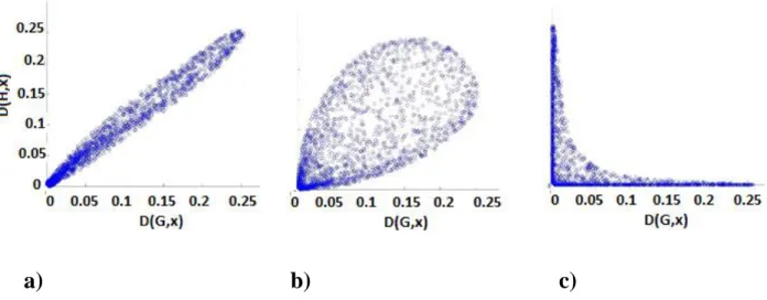
Li and Liu [2004] described a graphical approach called DD-plot (for depth-depth) to compare the 185
location of two subsamples. In the context of the T-test, a DD-plot consists in plotting (D) 186
DG1 x ,DG2 x
with x being from either subsample. When the two subsamples follow exactly187
the same distribution, the DD-plot is a diagonal line that passes through the origin as illustrated in 188
Figure 1a. However, if there is a location change, the graph has a form of leaf with its tip pointing 189
toward the origin (Figure 1b). The more important the location change is; the closer the tip will be 190
to the origin (Figure 1c). The T-test is based on an approximation of the distance between the tip 191
and the origin of the DD-plot. We define the set of points: 192
x ii| 1,...,n , there is no xj:DG1 xj DG1 xi and DG2 xj DG2 xi
(9)
193
Then we find the point xminof Ω such that: 194
1 min 2 min min 1 2
G G G G x D x D x D x D x
(10)
195If there are several points xmin, we take the mean of the corresponding coordinates. The point 196
identified by (10) is an approximation of the leaf-tip point of the DD-plot. The test statistic is then 197 given by: 198
G1 min G2 min
2 T D x D x(11)
199Even though, the distance of the leaf-tip to the origin is approximately 2T , the use of the statistic 200
T is equivalent. Similarly to the M-test, Li and Liu [2004] used the SD function (6) for the T-test. 201
However, MD (5) and TD (4) depths can also be used. The p-value is obtained using the Fisher’s 202
permutation test. 203
The W-test (Wilcox test) 204
The W-test was developed by Wilcox [2005]. Similarly to the M-test, the W-test is based on the 205
idea that under the null hypothesis, the medians of the two subsamples must be similar. To define 206
the W-test statistic, first the difference of each component is calculated 207
( ) ( ) ( )
, 1,..., ; 1,..., ; 1,...,
u u u
ij i j
d z y u d i s j m to constitute the vector dij
dij 1,,dij d
. 208Wilcox [2005] defined the test statistic by: 209 1,..., ; 1,..., ( ) max ( ) F F ij i s j m W D D d 0
(12)
210where F is the distribution of the set of vectors dijand D is the TD depth function (4). Under the 211
null hypothesis, we have W = 1, whereas under the alternative hypothesis, we have W < 1. The 212
asymptotic distribution of W is unknown. However, Wilcox [2005] proposed some critical values 213
Cfor significance levels 0.01; 0.025; 0.05; 0.10. The values of Care derived empirically
214
from simulations using a least squares regression method, and under the assumption of normality. 215
The null hypothesis is rejected when W is lower than C.
216
The QIA- and QIB-tests (quality index tests) 217
Liu and Singh [1993] developed a Wilcoxon-type rank test based on data depth. This test can detect 218
a location shift and/or a positive scale shift. The statistic of this test is given by: 219
m i i G G s a y y y D y D z n Q 1 1, , : # 1 (13)
220Under the null hypothesis, Qa = 0.5 whereas if there is a shift in location, then Qa < 0.5. Liu and
221
Singh [1993] used MD (5). Zuo and He [2006] found that under some regularity conditions, the 222
asymptotic distribution of Qa calculated with MD (5), TD (4) or projection depth is normal
223
2
,
N with mean 0.5 and variance 2
1 1
/12
s m
. In the present study, the 224
asymptotic (QIA-test) and bootstrap (QIB-test) methods are used to evaluate the p-values. 225
The Z-test (Zhang test) 226
Zhang et al. [2009] developed a new test based on the statistic Qa (13) where the statistic of the
Z-227
test is given by: 228
2 6 0.5 a Z s m Q n (14)
229To define Z, Zhang et al. [2009] used MD (5). To find the asymptotic distribution of Z, we define 230
the matrix A: 231
2 2 1 2 1 1 1 1 p p p p p p A
(15)
232 where pi = n ni, i = 1 or 2 and ni is the number of observations in the ith subsample. Let rbe the
233
rank of A, and the nonzero eigenvalues of A are denoted by λ1,..,λr. Under H0, Z follows
234
asymptotically a sum of independent chi-square distributions: 235
2 2 2
1 (1) 2 (1) ... r (1)
Z
(16)
236
This relation is also valid for the half-space and projection depth functions. The asymptotic method 237
is used to evaluate the corresponding p-value. 238
3.3. The p-value computation
239
The p-value of a given test is a simple criterion commonly used by practitioners to decide for the 240
acceptance or rejection of a target null hypothesis. The p-value is based on the distribution of the 241
statistics of the underlying test. For some of the considered tests in the present study, the asymptotic 242
or the exact distribution of the test statistic is unknown or difficult to obtain. Consequently, 243
approximations of the distribution of test statistics, under the null hypothesis, are required. To this 244
end, resampling methods are used. In the present paper, a permutation method [Snedecor and 245
Cochran, 1967] and a bootstrap method are used. They are briefly described below. More details 246
can be found, for instance, in Good [2005]. 247
To apply the permutation method, the observations should be exchangeable, i.e. the observations 248
should be independent and identically distributed [see e.g. Efron and Tibshirani, 1994]. This 249
method consists in permuting np times the sample
xi i1,...,n without replacement where np is a large250
number. For each permuted sample, the s first elements constitute the first subsample and the 251
remaining ones constitute the second subsample. The test statistic, generically denoted by S, is 252
calculated for each permutation
Si i*, 1,..., np
. The null hypothesis should be rejected for small values253
of the statistic. The p-value is the proportion of
*, 1,...,
p
i i n
S smaller or equal to the value Sobs
254
obtained from the original observed sample. 255
The bootstrap method is similar to the permutation method, except that the sample
1,... i i n
x is 256
resampled with replacement and the independence assumption is necessary [see e.g. Efron and 257
Tibshirani, 1994]. 258
3.4. Review of comparative studies
259
Some performance comparisons of the above tests are presented in the literature. The M- and T-260
tests, given respectively in (8) and (11), were compared to the Hotelling [1947] T2 test by Li and 261
Liu [2004]. The Hotelling’s T2 test is the most frequently used parametric test to detect location 262
shift [e.g. Ye et al., 2002]. For normally distributed samples with unit variances, the powers of 263
these three tests were found to be comparable, whereas for samples with Cauchy distribution with 264
the same parameter, the M- and T- tests were shown to be more powerful than the Hotelling’s test. 265
Moreover, in this case, the M-test outperformed the T-test. Note that both considered distributions 266
(normal and Cauchy) are symmetric. In order to evaluate the performance of these tests for skewed 267
distributions, Dovoedo and Chakraborti [2015] considered ten distributions belonging to five well-268
known families of multivariate skewed distributions. 269
Liu and Singh [2006] compared also the quality index test (13) to Hotelling’s test. For normal 270
samples, the performances of the two tests were similar, while for Cauchy and Exponential samples 271
the quality index test outperformed the Hotelling’s test. Baringhaus and Franz [2004] found that 272
the C-test (7) performs almost as well as Hotelling’s test for normal and non-normal samples. 273
These comparisons and evaluations are not appropriate for hydrological applications, since the 274
considered samples are not representative of the hydrological conditions where sample sizes are 275
generally short, and the variables mainly follow extreme distributions such as the Gumbel and the 276
Generalized Extreme Value (GEV) [e.g. El-Adlouni et al., 2010]. The Normal, Cauchy and t 277
distributions are not commonly used in multivariate HFA. In addition, in the literature, only partial 278
comparisons of the above tests were carried out and no overall comparison has been performed 279
dealing with all of them (to the best knowledge of the authors, the only references performing such 280
comparisons are those given in this section). 281
4. Simulation study
282
The objective of this simulation study is to evaluate and compare the performances of all the 283
previously presented tests in the hydrological context, such as in the case of flood series based on 284
flood peak Q and volume V. We also adopt samples with small sizes such as commonly 285
encountered in hydrology. 286
4.1. Adaptation to floods
287
The previously presented tests can be applied to hydrological events such as floods, rain storms 288
and droughts. In this paper, we focus on floods. Floods can be described by their peak Q, volume 289
V and duration D, which can be correlated. Indeed, according for instance to Yue [2001] there is 290
generally a strong correlation between Q and V, between V and D and a moderate correlation 291
between Q and D. In the present paper, the above considered tests are used to detect location shifts 292
in Q and V. These two variables are the most studied in hydrology for both the univariate and the 293
bivariate cases (see e.g. Chebana, 2013). 294
According to Sklar [1959], a bivariate distribution can be composed of marginal distributions and 295
a copula. Some previous studies showed that the Q and V series can be marginally fitted by a 296
Gumbel distribution [Chebana and Ouarda, 2007; Shiau, 2003; Yue, 2001; Yue et al., 1999]. The 297
cumulative Gumbel distribution is given by: 298
( ) exp exp x , and real, 0
F x x
(17)
299where x plays the role of each of the variables Q and V. The dependence between Q and V can be 300
represented by the Gumbel logistic model [e.g. Aissia et al., 2012; Chebana et al., 2009; Shiau, 301
2003; Yue et al., 1999], expressed according to the following copula: 302
1( , ) exp log( ) b log b b , 1 and 0 , 1
b
C u v u v b u v
(18)
303
Note that b1 1 where is the usual correlation coefficient [see e.g. Genest and Rivest, 304
1993; Gumbel and Mustafi, 1967]. 305
The presented tests may be affected by several factors. In the simulation study, we examine the 306
impact of the record length n (sample size) as well as the degree of change (shift amplitude) in each 307
component of the multivariate series. 308
For the simulation study, we generate samples (Q, V) according to models (17) and (18). We 309
consider the Gumbel distribution as marginal for both Q and V. The corresponding parameters are 310
denoted by: 311
- Q1and Q1 for respectively the scale and location parameters for Q of the first s observations 312
(before the shift); and 313
-Q2and Q2 for respectively the scale and location parameters for Q after the shift. 314
We define similarly the parameters of V
V, V
and the parameter b of the logistic Gumbel 315copula. 316
For the G distribution before the shift, we selected the parameters of the Skootamatta basin in 317
Ontario (Canada) which are also employed for simulation studies by Chebana and Ouarda [2007; 318
2009]. Consequently, Q1= 15.85, Q1= 51.85, V1= 300.22 V1 = 1239.8 and b = 1.414. Due to 319
space limitations, the reader is referred to the above references for more details regarding the 320
Skootamatta basin. 321
We study the effect of the following two factors on the performance of the tests: the record length 322
(n: sample size) and the amplitude of shifts in the location parameters, since the tests are mainly 323
designed to detect shifts in the location. Usually, the dependence parameter appears in the copula 324
whereas the location and scale parameters are present in the marginal distributions [Hobæk Haff et 325
al., 2010]. For location shift, we denote G1( )x =G2(x+) where δ = (δQ, δV) is the vector of the
326
shifts in the location of Q and the location of V respectively. In addition, the dependence level 327
between the two variables Q and V is considered with three dependence levels corresponding to 328
= 0.25 (low), = 0.50 (moderate) and = 0.75 (high) where the associated copula dependence 329
parameter is respectively b = 1.155, 1.414 and 2.0. 330
Even though the considered tests and the simulations are presented in the bivariate setting, they 331
can also be defined when more than two variables are involved to characterize the phenomenon. In 332
theory, the concepts of these tests can be extended to higher dimensions. However, some technical 333
difficulties could arise. First, the computation of some depth functions (which is the basis of a 334
number of the above tests) is complex and requires approximations and specific algorithms for 335
higher dimensions (e.g. for the simplicial depth). Second, a number of issues that are related to 336
models (especially for copulas) such as uncertainty increase, effectiveness of goodness-of-fit 337
testing, model formula complexity and questionable representativety of some models, need to be 338
addressed. Third, the number of the shift possibilities increases rapidly with the dimension, for 339
instance, with 3 variables we have 8 possibilities where the shift occurs without accounting for the 340
different shift amplitudes (for each variable) as well as the different types of dependence between 341
the variables (3 pairwise and 1 overall). Hence, the simulation results obtained in this paper cannot 342
be generalised directly to higher dimensions, and additional work will be required for this purpose. 343
4.2. Simulation design
344
The conducted simulation study consists of two steps. In the first one, we generate a large number 345
N of samples to evaluate the effects of different factors on the performance of the tests. Three 346
sample sizes are considered n = 30, 50 and 80 corresponding to s=5, 10; 5, 10, 20 and 5, 10, 20, 347
30 respectively. For each sample size, several amplitudes of location shift are considered: 𝛿= 10, 348
20, -20, 40 and 70%. We generate the samples as follows: 349
I. No change in all parameters: All the parameters of the distribution are the same before and 350
after the shift. This allows to obtain samples under the null hypothesis (no shift) and therefore, 351
for each record length n, we calculate the probability of type one error (α); 352
II. Change in location parameters: The distribution before the shift (G1) is the same as after the
353
shift (G2), except for the location parameters in the marginal. We consider 3 cases:
354
a. Change only in location of Q: ;
355
b. Change only in location of V: ;
356
c. Change in the location of Q and V simultaneously:
= (10,10), (20,20), (20,-20), Q, V
357
(40,40), and (70,70)%. 358
For the evaluation of p-values, based on the permutation and the bootstrap methods, we use np =
359
500 permutations or bootstrap samples. This value of np is proposed by Li and Liu [2004] for the
360
M- and T-tests and is superior to the value 200 proposed by Baringhaus and Franz [2004] for the 361 C-test. 362 = 10, 20, 40 and 70% Q 10, 20, 40 and 70% V
In the second step of the simulation study, we evaluate the performance of each test on the basis of 363
the estimate ˆ of the type one error α and the power of the considered tests. In the present study, 364
we fix α = 5%. Consequently, we reject H0 if the p-value is less than 5%. We consider a number of
365
replications N=3000 which higher than the number of replications used by Li and Liu [2004], 366
Wilcox [2005] and Zhang et al. [2009]. 367
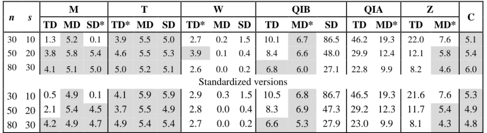
Since the peak and the volume have very different scales, we also considered standardizing the 368
generated samples (with the known standard deviation and its empirical estimate of the whole 369
sample before and after the shift). Note that the standard deviation of a Gumbel distribution can be 370
obtained directly from its scale parameter
as 6. 3714.3. Simulation results
372
In order to avoid repetition and for notation simplicity, the depth function will only be written in 373
the test index when it is needed. For example, MTD-test is the M-test with TD depth function.
374
I. Type one error estimation 375
The estimates ˆ of α for the considered tests are presented in Table 2 (with and without 376
standardization). First, we observe that the results are almost the same with and without 377
standardization for all situations and tests. Since the critical level is fixed at α = 5%, a performing 378
test should have ˆ as close as possible to 5%. From Table 2, we see that ˆ generally approaches 379
5% when n increases. Values of ˆ for the M-test are close to 5% except for MTD and MSD in the
380
case (n,s)=(30,10). The T- and C-tests have ˆ around 5% whatever the sample size. The W-test 381
underestimates α while the QIB-, QIA- and Z-tests overestimate it. However, the QIBSD-, QIATD-
382
and ZTD- tests have ˆ higher than 20% when (n,s)=(30,10) which means that they reject H0 more
383
frequently when it is true. 384
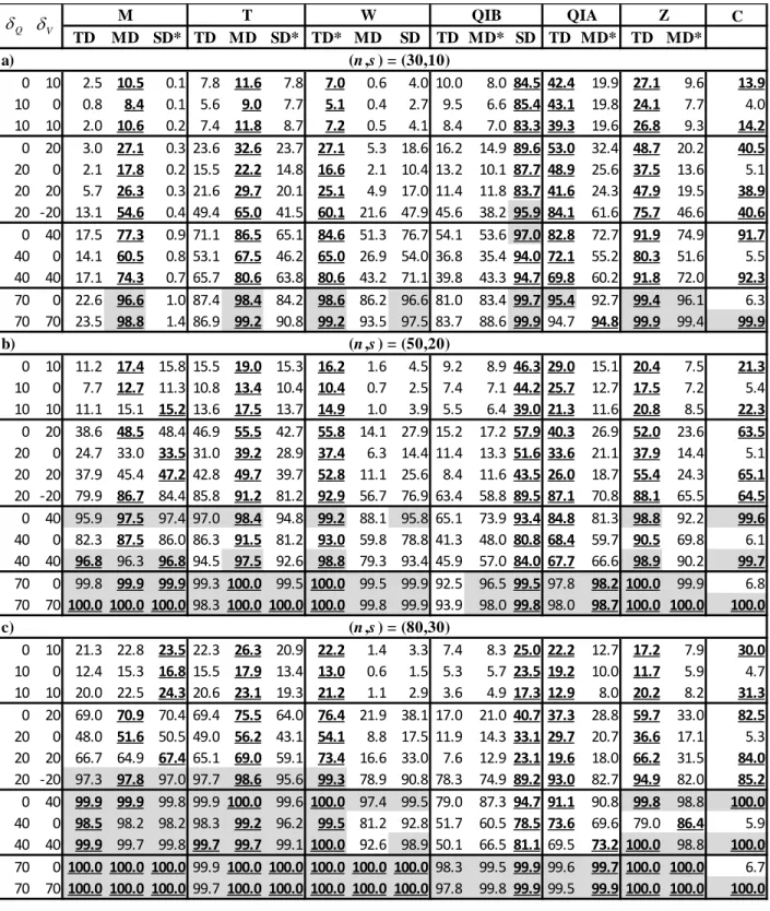
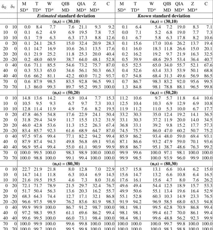
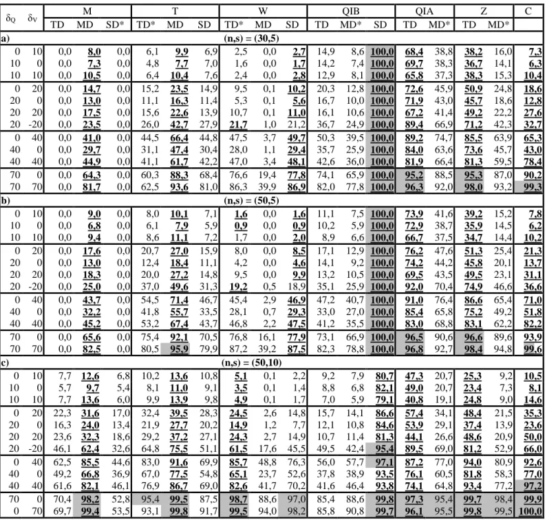
II. Power evaluation 386
Table 3 summarises the simulation results for shift detection tests for several shift amplitudes in Q, 387
V and (Q,V). In general, these results show good behaviour for the tests in terms of power. The 388
power increases with the shift amplitude 𝛿 and with the sample size n. In the present paper, a test 389
power is considered high when it exceeds 95%. 390
For n=30, Table 3 (part a) shows that high powers are generally recorded for large shift amplitudes 391
i.e.
= (70,0) or Q, V
= (70,70). For the M- and T-tests, best powers are recorded Q, V
392with the MD depth function. The TD depth function gives best powers for the W-, QIA- and Z-393
tests while for the QIB-test, the best power is reached with the SD depth function. However, as 394
seen before, the QIBSD-, QIATD- and ZTD-tests are problematic when estimating α. Note that the
395
depth function that provides the best test power is not necessarily the one with which the test was 396
originally defined, e.g. M- and T-tests. For the C-test, the power depends on the variable in which 397
the shift has occurred. Indeed, a shift only in Q leads to low power for the C-test, while the opposite 398
is true when the shift is either in V or in (Q,V). This is due to the difference in the first term in (7) 399
which can be affected by the scale of the series. In the case of floods, Q and V series have very 400
different scales. Consequently, a change in Q does not have a great effect on the test statistic while 401
the opposite is true for V (and hence for (Q,V)). We can conclude that the C-test is more sensitive 402
to a change in V than a change in Q. This result was not shown in previous studies since the 403
simulations were based on variables of the same nature and scale. This can be explained by the fact 404
that the statistic C is based on the Euclidian distance which is not affine invariant whereas the 405
depth-based tests are not affected by the scale since depth functions are usually affine invariant 406
[Zuo and Serfling, 2000]. 407
For n = 50, from Table 3 (part b), we can see that high powers are obtained starting form
Q, V
408= (0,40). For each test, the depth functions that lead to the best power when n = 30 are generally 409
the same when n=50. The powers when n=50 are generally higher than the power corresponding 410
to n=30 with a few exceptions: for QIB-, QIA-, and Z-tests with
=(0,10), (10,0), (10,10), Q, V
411(0,20), (20,0) or (20,20). 412
Table 3 (part c) summarizes the simulation results of the presented tests when n=80. Results show 413
that high powers are observed starting from
= (20,-20) for the M-, T- and WQ, V
TD-tests. For414
the M-test, results are similar for the three considered depth functions for each shift amplitude 415
whereas for the other tests, depth functions leading to the highest powers for n=80 are also the 416
same as for n=30 or 50. Generally, the performances of the tests increase when the shifts of V and 417
Q have different signs. For instance, the powers for
= (20,-20) are higher than those Q, V
418corresponding to
= (20, 20) for all tests. Note that the C-test power increases with n except Q, V
419when the shift is located only in Q. 420
From these results one can conclude that, generally, best results are obtained by the M-, T- and W-421
tests (with power higher or equal to that of the rest of the tests). For low sample sizes, high powers 422
are observed for large shift amplitudes (70%), while for large sample sizes, high powers are 423
observed starting from
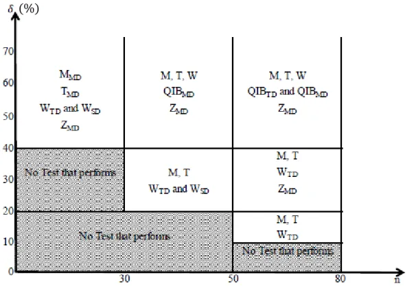
=(20,-20)%. For low shift amplitudes (10%), low powers are Q, V
424recorded for all the considered tests. Figure 2 illustrates the applicability (where power is 425
reasonable or high) of considered tests for the combinations of the studied sample sizes and shift 426
amplitudes. 427
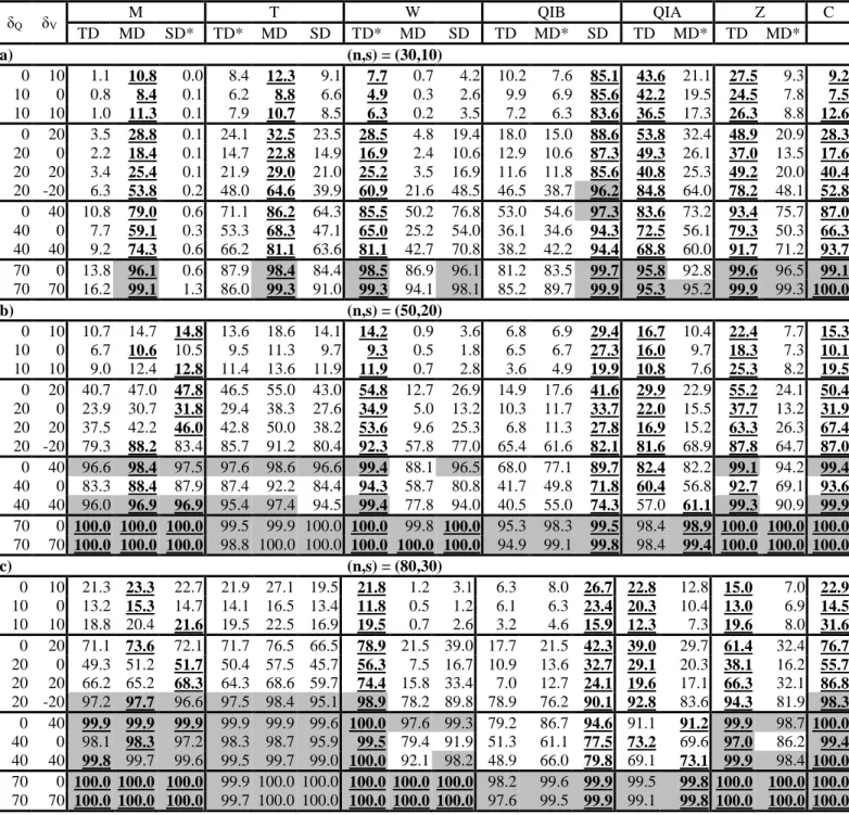
As shown in Table 3, the powers of the tests, in particular the C-test, are affected by the different 428
scales in the variables V and Q. Table 4 presents results corresponding to the case when the 429
generated series are standardized using the corresponding estimated standard deviation. We 430
observe that the standardized C-test provides better results especially when the change is 431
symmetrical in V or in Q, such as the case
= (0,20) or (20,0)%. However, it is still affected Q, V
432in the sense that the power is not the same when the variables are affected symmetrically. The other 433
tests remain almost the same after standardization even though the power is reduced for some tests 434
(e.g. QIB_SD, QIA, n=50). 435
In Table 5, we consider standardizing with the estimated or known standard deviation. We observe 436
from Table 5 that the power is close to being symmetric regarding the change in V or Q when the 437
standard deviation is estimated, and the power becomes almost symmetric when the standard 438
deviation is known. The improvement is increasing with the sample size where, for instance, the 439
power is almost identical when a change affects either V or Q with the same shift magnitude. Note 440
that by construction, the depth-based tests should not be affected by the scale since the depth 441
functions are affine-invariant (see Li and Liu, 2004). 442
Table 6 presents evaluations of the power of the previous tests (with standardized samples) with 443
different possibilities of the location of the shift through different values of s. We observe that for 444
a given n, the power generally increases with s, with some exceptions such as for QIA and QIB for 445
which the power decreases with s. We observe also that small values of s (mainly s = 5 in the 446
present study) affect the depth computations of some tests like the M and QIB tests which presented 447
unexpected behaviors (always 0% for M or 100% for QIB). 448
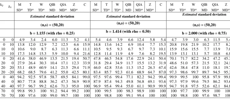
Variations of the type one error (α) estimations and the power with respect to the dependence level 449
are presented in Table 7. Regarding α estimation, for a given test, the estimation is practically 450
unaffected for all three dependence levels. Regarding the power, in general for all depth-based 451
tests, the power is increasing with some exceptions related to the values of δQ and δV, such as (0,10)
452
and (10,10). The C-test seems to be almost unaffected by the dependence level. 453
During the simulation, a problem related to the set Ω occurred with the T-test. Indeed, the set Ω 454
given in (9) can be empty. It was observed that Ω is rarely empty in general with the SD and MD 455
depths, but it is often empty with the TD depth. This issue was not mentioned or considered in Li 456
and Liu [2004]. These cases are excluded from the present computations. 457
From the present simulation study, the following general observations can be made (also illustrated 458
in Figure 2): 459
- The C-test is more sensitive to a change in V than a change in Q; 460
- For a small sample size (n=30), high power is observed only for high shift amplitudes; 461
- For a large sample size (n=80), best powers are observed for the M-, T- and W-tests; 462
- The QIB-, QIA- and Z-tests can be problematic especially for low shift amplitudes; 463
- For type one error estimation, QIBSD-, the QIA- and ZTD-tests are problematic, especially
464
when n=30. Good performances are observed for the M-, T-, W- and C-tests with all depth 465
functions; 466
- For low shift amplitudes
= (0, 10), (10, 0) or (10, 10), powers are low. This means Q, V
467that a 10% change in one or both location parameters is not detected by the considered tests; 468
- The C-test is severely affected by the scale and samples should be standardized to reduce 469
this effect. However, the depth-based tests are less affected by the variable scale; 470
- Generally, the power increases with the location shift s. However, some tests provided 471
inconsistent results when s is very close to the beginning (or the end) of the series; 472
- Generally the power of the depth-based tests increases with the dependence level whereas 473
the C-test is almost unaffected by this factor. 474
5. Application
475
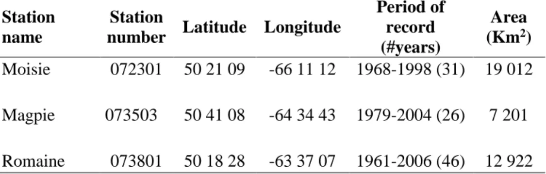
In this section, the previously considered tests are applied to the data series of three stations 476
(Moisie, Magpie and Romaine) with natural flow regimes. Moisie and Romaine are among a 477
number of stations selected in Canada to be part of the Reference Hydrometric Basin Network 478
(RHBN) used for the study of the impacts of climate change on hydrologic regimes in the country 479
[Ouarda et al. 1999]. The three considered stations are located in the Cote Nord Region of the 480
province of Quebec, Canada. The Moisie station (reference number 072301) is located on Moisie 481
River at 1.5 km upstream of the Québec North Shore Labrador Railway (QNSLR) bridge with a 482
drainage basin area of 19 012 km2. Data series are available from 1968 to 1998. The Magpie station 483
(reference number 073503) is located at the outlet of Magpie Lake. Its drainage basin has an area 484
of 7 201 km2 and observations are available from 1979 to 2004. The Romaine station (reference 485
number 073801) is located at 16.4 km from the Chemin-de-fer bridge on Romaine River, with a 486
drainage basin area of 12 922 km2 and available data from 1961 to 2006. Figure 3 and Table 7 487
present respectively the geographical location and general information about the considered 488
stations. 489
Spring flood characteristics Q and V are extracted from daily streamflow series for each station. 490
The peak Q is defined as the maximum annual of daily streamflow series whereas the volume V is 491
the cumulative streamflow over the flood event, see e.g. Aissia et al. [2012] for formal definitions 492
of flood variables. Note that the variables Q and V correspond to the same flood event each year. 493
In particular, they correspond to the annual spring flood event which is generally the important 494
flood event in the year and is caused mainly by snow melting [Aissia et al., 2012]. 495
Figure 4 shows the time series of Q and V for the three stations. Since these stations are 496
geographically close to each other (Figure 3), it is expected that any eventual shift would be 497
observed in all three stations. From Figure 4 we can see that a shift can be located in Q and V 498
around 1984 for all three stations. Therefore, the previously presented tests (with and without 499
standardizing the samples) are applied for each station in 1984. Statistics and p-values of the 500
considered tests are summarized in Table 8. Note that, instead of the p-value, for the W-test the 501
conclusion is presented as: 1 if there is a shift, 0 if not, since this test is based on critical thresholds 502
[Wilcox, 2005]. 503
First, we observe that the standardization does not affect the values of the test statistics of the depth-504
based tests whereas the C-test statistics are completely different. However, the p-values are almost 505
the same and the standardization generally does not change the conclusions. Results show that all 506
considered tests are in agreement with the existence of a shift in the Moisie station data. For 507
instance, the p-values of the T-, QIB-, QIA-, Z- and C-tests are less than 1%. For Magpie station, 508
the M-test is the only test which does not detect the presence of a shift for all depth functions 509
whereas the T-test indicates a shift with all depth functions. This can be explained by the fact that 510
for small sample sizes (Table 3a) the power of the M-test is lower than the power of the T-test. 511
Considering Romaine station, only the TSD-, QIBTD-, QIBMD- and ZTD-tests cannot confirm the
512
existence of a shift in the year 1984. 513
From the results of the three stations, one can conclude that, the year 1984 is detected as a shift for 514
the Moisie station by all tests (and depth functions) and for Romaine station by all tests (not all 515
depth functions). However, for the Magpie station, 3 out of 6 tests detect the shift. Indeed, from 516
Figure 4b one can see that a shift in 1984 is not very clear in Magpie station and the short sample 517
data before the shift can have an impact on the power of considered tests. Since these stations are 518
geographically close (Figure 3), one can say that 1984 represents probably a shift for all these 519
stations. 520
6. Conclusions
521
The aim of this paper is to study shift detection in the multivariate hydrological setting by 522
comparing the power of several tests and by adapting these tests for hydrological practice. Shift 523
detection is required to insure the validity of HFA assumptions (homogeneity and stationarity) and 524
has hence a strong impact on the selection of the appropriate multivariate distribution. All 525
considered tests are based on data depth, except for the C-test, which is considered for comparison 526
purposes. An overall simulation study that considers all the considered tests and which takes into 527
account the hydrological context, is performed to evaluate and compare the power of the considered 528
tests to detect shifts in the location parameter of Q, V and (Q,V). These tests are also applied to a 529
real-world flood case study consisting of three stations from the province of Québec, Canada. 530
In general, the powers of these tests increase with the shift amplitude and with the sample size. 531
However, the QIA-, QIB- and Z-tests may be problematic for small sample sizes and they 532
overestimate the type one error α. The scale of the tested variables has an effect on the performance 533
of the considered tests. Especially, the C-test is severely affected and requires a standardizing of 534
the samples. In general, the tests are more powerful when the shift occurs far from the end or the 535
beginning of the series. For low shift amplitudes, the considered tests do not perform well for all 536
sample sizes. On the basis of the above comparison, and considering the nature of hydrological 537
data, it can be recommended to use the M-, T- and W-tests. More precisely, for small sample sizes, 538
the MD depth function is preferred for the M- and T-tests while the TD depth function is preferred 539
for the W-test whereas TD and SD are not recommended when testing a shift far from the middle 540
section of the series. 541
The application of the considered tests to observed hydrological data shows their ability to detect 542
multivariate shifts. It is also observed that the performance of the tests is affected by the length of 543
the sub-series before or after the shift. The current literature review and hydrologic simulations and 544
application focused on the bivariate cases. It is recommended to examine the performance of these 545
tests for higher dimensions in future research efforts. 546
ACKNOWLEDGEMENTS
547
The authors are grateful to the Editor, the Associate Editor and the reviewers for their comments 548
and suggestions which helped improve the quality of the paper. The authors thank the Natural 549
Sciences and Engineering Research Council of Canada (NSERC) for the financial support and 550
Marjolaine Dubé for her assistance. 551
References
552
Aissia, M. A. B., F. Chebana, T. B. M. J. Ouarda, L. Roy, G. Desrochers, I. Chartier, and É. 553
Robichaud (2012), Multivariate analysis of flood characteristics in a climate change context of the 554
watershed of the Baskatong reservoir, Province of Québec, Canada, Hydrological Processes, 26(1), 555
130-142. 556
Baringhaus, L., and C. Franz (2004), On a new multivariate two-sample test, Journal of 557
Multivariate Analysis, 88(1), 190-206. 558
Beaulieu, C., T. B. M. J. Ouarda, and O. Seidou (2007), A review of homogenization techniques 559
for climate data and their applicability to precipitation series, Hydrological Sciences Journal, 560
52(1), 18-37. 561
Beaulieu, C., O. Seidou, T. B. M. J. Ouarda, X. Zhang, G. Boulet, and A. Yagouti (2008), 562
Intercomparison of homogenization techniques for precipitation data, Water Resources Research, 563
44(2), W02425. 564
Beaulieu, C., Seidou, O., Ouarda, T.B.M.J., and X. Zhang (2009). Intercomparison of 565
homogenization techniques for precipitation data continued: Comparison of two recent Bayesian 566
change point models, Water Resources Research, 45, W08410, doi:10.1029/2008WR007501. 567
Beaulieu, C., Ouarda, T.B.M.J., and O. Seidou. (2010). A Bayesian Normal Homogeneity Test for 568
the detection of artificial discontinuities in climatic series, International Journal of Climatology, 569
DOI: 10.1002/joc.2056. 570
Bobée, B., and F. Ashkar (1991), The gamma family and derived distributions applied in 571
hydrology, Water Resources Publication. Littleton, Colorado, USA. 572
Bowman, A. W., A. Pope, and B. Ismail (2006), Detecting discontinuities in nonparametric 573
regression curves and surfaces, Statistics and Computing, 16(4), 377-390. 574
Burn, D. H., and M. A. Hag Elnur (2002), Detection of hydrologic trends and variability, Journal 575
of Hydrology, 255, 107–122. 576
Chebana, F. (2013), Multivariate Analysis of Hydrological Variables, in Encyclopedia of 577
Environmetrics, edited, John Wiley & Sons, Ltd. 578
Chebana, F., and T. B. M. J. Ouarda (2007), Multivariate L-moment homogeneity test, Water 579
Resources Research, 43(8). 580
Chebana, F., and T. B. M. J. Ouarda (2008), Depth and homogeneity in regional flood frequency 581
analysis, Water Resources Research, 44(11). 582
Chebana, F., and T. B. M. J. Ouarda (2009), Index flood–based multivariate regional frequency 583
analysis, Water Resources Research, 45(10), W10435. 584
Chebana, F., and T. B. M. J. Ouarda (2011), Multivariate quantiles in hydrological frequency 585
analysis, Environmetrics, 22(1), 63-78. 586
Chebana, F., T. B. M. J. Ouarda, and T. C. Duong (2013), Testing for multivariate trends in 587
hydrologic frequency analysis, Journal of Hydrology, 486(0), 519-530. 588
Chebana, F., T. B. M. J. Ouarda, P. Bruneau, M. Barbet, S. El Adlouni, and M. Latraverse (2009), 589
Multivariate homogeneity testing in a northern case study in the province of Quebec, Canada, 590
Hydrological Processes, 23(12), 1690-1700. 591
Chen, S., Li, Y., Kim, J. and Kim, S. W. (2016), Bayesian change point analysis for extreme daily 592
precipitation. Int. J. Climatol.. doi:10.1002/joc.4904 593
Cramér, H. (1928), On the composition of elementary errorsé: II, Statistical applications, 594
Skandinavisk Aktuarietidskrift, 11, 141-180. 595
Deng, J. L. (1989), Introduction to Grey System Theory, J. Grey Syst., 1(1), 1-24. 596
Dovoedo, Y.H. and Chakraborti, S. (2015), Power of depth-based nonparametric tests for 597
multivariate locations, Journal of Statistical Computation and Simulation, 85:10, 1987-2006 598
Easterling, D. R., and T. C. Peterson (1995), A new method for detecting undocumented 599
discontinuities in climatological time series, International Journal of Climatology, 15(4), 369-377. 600
Efron, B., and R. J. Tibshirani (1994), An Introduction to the Bootstrap, Taylor & Francis. 601
El Adlouni, S., Chebana, F., and Bobée, B. (2010), Generalized Extreme Value versus Halphen 602
System: Exploratory Study. J. Hydrol. Eng., 10.1061/(ASCE)HE.1943-5584.0000152, 79-89. 603
Ehsanzadeh, E., Ouarda, T. B. M. J. and Saley, H. M. (2011), A simultaneous analysis of gradual 604
and abrupt changes in Canadian low streamflows. Hydrol. Process., 25: 727–739. 605
doi:10.1002/hyp.7861 606
Genest, C., and L.-P. Rivest (1993), Statistical Inference Procedures for Bivariate Archimedean 607
Copulas, Journal of the American Statistical Association, 88(423), 1034-1043. 608
Good, P. (2005), Permutation, Parametric and Bootstrap Tests of Hypotheses, 315 pp., Springer 609
New York. 610
Gumbel, E. J., and C. K. Mustafi (1967), Some Analytical Properties of Bivariate Extremal 611
Distributions, Journal of the American Statistical Association, 62(318), 569-588. 612
Hobæk Haff, I., K. Aas, and A. Frigessi (2010), On the simplified pair-copula construction — 613
Simply useful or too simplistic?, Journal of Multivariate Analysis, 101(5), 1296-1310. 614
Hotelling, H. (1947), Multivariate quality control: Illustrated by the air testing of sample bomb 615
sight., in In Selected Techniques of Statistical Analysis for Scientific and Industrial Research and 616
Production and Management Engineering, edited by McGraw-Hil, pp. 111-184, New York. 617
Jandhyala, V., P. Liu, S. Fotopoulos, and I. MacNeill, (2014) Change-Point Analysis of Polar Zone 618
Radiosonde Temperature Data. J. Appl. Meteor. Climatol., 53, 694–714,doi: 10.1175/JAMC-D-619
13-084.1. 620
Kao, S.-C., and R. S. Govindaraju (2007), A bivariate frequency analysis of extreme rainfall with 621
implications for design, J. Geophys. Res., 112(D13), D13119. 622
Lee, T.-S., Ouarda, T.B.M.J., Chebana, F., and D. Park (2014), Evaluation of a Depth-Based 623
Multivariate -Nearest Neighbor Resampling Method with Stormwater Quality Data, Mathematical 624
Problems in Engineering, 2014 (404198), doi:10.1155/2014/404198. 625
Li, J., and R. Y. Liu (2004), New Nonparametric Tests of Multivariate Locations and Scales Using 626
Data Depth, Statistical Science, 19(4), 686-696. 627
Lin, L., and M. Chen (2006), Robust estimating equation based on statistical depth, Statistical 628
Papers, 47(2), 263-278. 629
Liu, R. Y. (1990), On a Notion of Data Depth Based on Random Simplices, The Annals of 630
Statistics, 18(1), 405-414. 631
Liu, R. Y., and K. Singh (1993), A Quality Index Based on Data Depth and Multivariate Rank 632
Tests, Journal of the American Statistical Association, 88(421), 252-260. 633
Liu, R. Y., and K. Singh (2006), Rank tests for multivariate scale difference based on data depth, 634
in Data Depth: robust multivariate analysis, computational geometry, and applications, edited by 635
R. Y. S. Liu, K. and Souvaine, D.L., pp. 17-35, Àmerican Mathematical Society. 636
Lund, R., and J. Reeves (2002), Detection of Undocumented Changepoints: A Revision of the Two-637
Phase Regression Model, Journal of Climate, 15(17), 2547-2554. 638
Mizera, I., and C. H. Müller (2004), Location-scale depth, Journal of the American Statistical 639
Association, 99(468), 949-966. 640
Moore, R. E. (1979), Methods and Applications of Interval Analysis, SIAM, Philadelphia, USA. 641
Naizghi, M. S., and T. B. M. J. Ouarda (2016). Teleconnections and analysis of long-term wind 642
speed variability in the UAE, International Journal of Climatology, DOI: 10.1002/joc.4700. 643
Ouarda, T. B. M. J. and S. El-Adlouni (2011). Bayesian nonstationary frequency analysis of 644
hydrological variables. Journal of the American Water Resources Association (JAWRA), 1-10, 645
47(3): 496-505. DOI: 10.1111/j.1752-1688. 646
Ouarda, T., M. Haché, P. Bruneau, and B. Bobée (2000), Regional Flood Peak and Volume 647
Estimation in Northern Canadian Basin, Journal of Cold Regions Engineering, 14(4), 176-191. 648
Ouarda, T.B.M.J., Rasmussen, P.F., Cantin, J.F., Bobée, B., Laurence, R., Hoang, V.D. and G. 649
Barbé (1999). Identification of a hydrometric data network for the study of climate change over 650
the province of Quebec. Revue des Sciences de l’eau, 12(2): 425-448. 651
Ouarda, T.B.M.J., Charron, C., Niranjan Kumar, K., Marpu, P., Ghedira, H., Molini, A.L., Khayal 652
(2014). Evolution of rainfall regime in the UAE, Journal of Hydrology, 514 (June): 258–270, 653
DOI:10.1016/j.jhydrol.2014.04.032. 654
Peterson, T. C., et al. (1998), Homogeneity adjustments of in situ atmospheric climate data: A 655
review, International Journal of Climatology, 18(13), 1493-1517. 656
Rao, A. R., and K. H. Hamed (2000), Flood Frequency Analysis, CRC Press, Boca Raton. 657
Sagarin, R., and F. Micheli (2001), Climate change in nontraditional data sets, Science, 294(5543), 658
811. 659
Seidou, O., and T.B.M.J., Ouarda (2007). Recursion-based multiple changepoint detection in 660
multivariate linear regression and application to river streamflows, Water Resources Research. 43, 661
W07404, doi:10.1029/2006WR005021, 1-18. 662
Seidou, O., J. J. Asselin, and T. B. M. J. Ouarda (2007), Bayesian multivariate linear regression 663
with application to change point models in hydrometeorological variables, Water Resources 664
Research, 43(8),. 665
Shiau, J. T. (2003), Return period of bivariate distributed extreme hydrological events, Stochastic 666
Environmental Research and Risk Assessment, 17(1-2), 42-57. 667
Singh, S. K., and A. Bárdossy (2012), Calibration of hydrological models on hydrologically 668
unusual events, Advances in Water Resources, 38(0), 81-91. 669
Sklar, A. (1959), Fonctions de ré partition à n dimensions et leurs marges. 670
Snedecor, G. W., and W. G. Cochran (1967), Statistical Methods, Iowa State University Press. 671
Solow, A. R. (1987), Testing for Climate Change: An Application of the Two-Phase Regression 672
Model, Journal of Climate and Applied Meteorology, 26(10), 1401-1405. 673