Dynamics of a hybrid morphing wing with active open loop vibrating trailing edge by Time-Resolved PIV and force measures

(1)

To link to this article : DOI:

10.1016/j.jfluidstructs.2017.06.015

URL : https://doi.org/10.1016/j.jfluidstructs.2017.06.015

This is an author-deposited version published in:

http://oatao.univ-toulouse.fr/

Eprints ID: 16095

Open Archive Toulouse Archive Ouverte (OATAO)

OATAO is an open access repository that collects the work of Toulouse

researchers and makes it freely available over the web where possible.

To cite this version: Jodin, Gurvan and Motta, Valentina and Scheller,

Johannes and Duhayon, Eric and Döll, Carsten and Rouchon,

Jean-François and Braza, Marianna Dynamics of a hybrid morphing wing with

active open loop vibrating trailing edge by Time-Resolved PIV and force

measures. (2017) Journal of Fluids and Structures, vol. 74. pp. 263-290.

ISSN 0889-9746

Any correspondence concerning this service should be sent to the repository administrator:

(2)

Dynamics of a hybrid morphing wing with active open loop

vibrating trailing edge by time-resolved PIV and force

measures

G. Jodin

a,c,

*

,1

_{, V. Motta}

b,2

_{, J. Scheller}

c,d,2

_{, E. Duhayon}

a,3

_{, C. Döll}

b,4

_,

J.F. Rouchon

a,5

, M. Braza

c,

*

,6

a_{Laboratoire Plasma et Conversion d’Énergie (LAPLACE), UMR 5213 CNRS-INPT-UPS, 2, rue Charles Camichel, 31071 Toulouse, France} b_{ONERA - System Control and Flight Dynamics Department, 2 av. Edouard Belin, 31055 Toulouse, France}

c_{Institut de Mécanique des Fluides de Toulouse (IMFT), UMR 5502 CNRS-INPT-UPS, Allée du prof. Camille Soula, 31400 Toulouse, France} d_{Massachusetts Institute of Technology (MIT), 77 Massachusetts Ave, Cambridge, MA 02139, United States}

Keywords: Morphing Smart materials Wind tunnel experiments Vortex breakdown Harmonic forcing

a b s t r a c t

A quantitative characterization of the effects obtained by high frequency–low amplitude trailing edge actuation is presented. Particle image velocimetry, pressure and aerody-namic forces measurements are carried out on a wing prototype equipped with shape memory alloys and trailing edge piezoelectric-actuators, allowing simultaneously high deformations (bending) in low frequency and higher-frequency vibrations. The effects of this hybrid morphing on the forces have been quantified and an optimal actuation range has been identified, able to increase lift and decrease drag. The present study focuses more specifically on the effects of the higher-frequency vibrations of the trailing edge region. This actuation allows manipulation of the wake turbulent structures. It has been shown that specific frequency and amplitude ranges achieved by the piezoelectric actuators are able to produce a breakdown of larger coherent eddies by means of upscale energy transfer from smaller-scale eddies in the near wake. It results a thinning of the shear layers and the wake’s width, associated to reduction of the form drag, as well as a reduction of predominant frequency peaks of the shear-layer instability. These effects have been shown by means of frequency domain analysis and Proper Orthogonal Decomposition.

*

Corresponding authors.

E-mail addresses:[email protected](G. Jodin),[email protected](V. Motta),[email protected](J. Scheller),

[email protected](E. Duhayon),[email protected](C. Döll),[email protected](J.F. Rouchon),[email protected]

(M. Braza). 1 _{PhD fellow.} 2 _{Postdoctoral fellow.} 3 _{Associate professor.} 4 _{Senior research scientist.} 5 _{Full Professor.}

(3)

Nomenclature

u2_,

_v

2 _{Time average of the stream-wise and crossflow component of the Reynolds tensor.}

A, a∗ _{HFVTE actuation amplitude (mm). a}∗

₌

A

c is the dimensionless amplitude. c Chord length

D, D, CD Drag force, time average drag, drag coefficient CD

=

D

1/2SρU2

∞

. With

ρ

the air density, S the reference wing section.

Fa, fa∗ HFVTE actuation frequency (Hz), dimensionless actuation frequency fa∗

=

U∞Fac L, L, CL Lift force, time average lift, lift coefficient CL

=

₁_/_2SL_ρ_U2

∞. With

ρ

the air density, S the reference wing section.

St Strouhal number. St

=

_U∞f·c, with f the frequency in Hz.

u,

v

Stream-wise (u), respectively crossflow (

v

) fluctuating component of the flow velocity normalized in relation with U∞. u

=

U

−

U,

v =

V

−

V

U, V and U, V Stream-wise (U), and crossflow (V ) component of the flow velocity normalized in relation with U∞.

U, V are the time averages of the components. U∞ Free stream velocity (m/s)

HFVTE Higher Frequency Vibrating Trailing Edge MFC Piezoelectric Macro-fiber Composite Patches. POD Proper Orthogonal Decomposition.

PSD Power Spectral Density.

Re Reynolds number relative to the chord c. Re

=

cU∞_ν where

ν

is the kinematic viscosity of the air. Sk Stokes number, Sk

=

ρρ d

2

ρ U∞

18µδc , where

µ

is the dynamic viscosity of the fluid,

ρ

ρis the density of the smoke

particles,

δ

cis the characteristic length i.e. the model chord and dρis the diameter of the particles

SMA Shape Memory Alloy.

TNT Turbulent/Non Turbulent Interfaces TRL Technology Readiness Level

1. Introduction

Limiting energy consumption has become a central concern for reducing aircraft operational costs. Improving aerody-namic performance is a way to reduce the fuel burn during flight.

Current airfoil shapes are generally optimized for only a few flight states, corresponding to nominal cruise conditions. During flight, the altitude, the weight and the speed are continuously changing. Hence this design is sub-optimal for the whole aircraft mission. Traditional solutions to control and adapt the wing shape (like slats and flaps) exhibit limited performance ranges (Barbarino et al., 2011). Changing the shape of the wing during a mission can save several percents of fuel for a regional passenger aircraft (Zhoujie, and Martins, 2015). The concept of real time shape and vibrational behavior adaptation enabling multi-point optimization is called morphing. In the context of the studies carried out in the authors multi-disciplinary research platform involving the LAPLACE and IMFT French Laboratories,7 _{the morphing is achieved by}

means of electro-actuation and is called ‘‘electroactive morphing’’.

Within the framework of aircraft aerodynamic performance, it was demonstrated that camber control of the trailing edge of a wing is very efficient to improve aircraft performance (Lyu and Martins, 2015). With this regard relatively high Technology Readiness Level (TRL) projects, targeting current industrial airliners at true scale, were undertaken. The European research programs SARISTU8 and CleanSky9 have work packages dealing with morphing wing trailing edge devices,Dimino et al.(2016) andPecora et al.(2016). Another trailing edge morphing concept, called Adaptive Compliant Trailing Edge, was developed by NASA in cooperation with FlexSys Inc.10 _{This concept features an adjustable structure which can be actively}

deformed. Endurance flight tests for this concept were performed and described inKota et al.(0000). This solution was proved to yield aerodynamic benefits and its effectiveness and airworthiness are being ultimately assessed.

However these new adaptive structures are actuated through conventional actuators like servomotors. Recent advances in the field of smart materials show the potential to overcome difficulties to make a wing both stiff enough to withstand the loads, and flexible enough to be easily deformed (Barbarino et al., 2014). The related research focuses mainly on low scale Micro Air Vehicles. Among electro-active materials, Shape Memory Alloys (SMAs) and piezoelectric materials are the most frequently used. SMAs are characterized by thermo-mechanical behaviors, and most applications use Joule heating to

7 _{http://www.smartwing.org/}_. 8 _{http://www.saristu.eu}_. 9 _{http://www.cleansky.eu/}_. 10 _{http://www.flxsys.com/}_.

(4)

activate the SMAs. Different morphing concepts were developed, an overview of which is presented by Barbarino et al. in

Barbarino et al.(2011). The electromechanical response of piezoelectric materials is activated via the application of an electric field (Barbarino et al., 2014). The material commonly employed is Lead Zirconate Titanate (LZT or PZT) ceramic. Piezoelectric composites allow for a simple implementation. Piezoelectric composite patches glued on structure are often used as bending actuators to control the wing shape. The desired operation is generally accomplished using one specific smart material. A combination of both SMAs and LZT can enhance significantly the global performance. The synergistic smart morphing aileron (Pankonien et al., 2015) is the combination of a SMA actuated hinge followed by a flexible piezoelectric driven trailing edge. The works mentioned above deal with global airflow control to improve macroscopic behavior i.e. lift, drag, aeroelastic response, or load alleviation by means of quasi static shape control. A dynamic flow control is also possible. For example

Grigorie et al.(0000) presents a wind tunnel model with shape adaptive upper side. Two SMA actuators control the airfoil

thickness, whereas pressure sensors are used to estimate the location of the separation point. The work of Inaoka et al. in

Inaoka et al.(2015) deals with active vibrating flaps located on the leading edge. These flaps are actuated at a frequency corresponding to the vortex generation frequency of vortices in the separated area. This control allows for avoiding the flow separation when a decrease in free stream velocity occurs. Vibrating trailing edge concepts are also studied for rotorcraft applications. Large coherent flow instabilities have been modeled and then open and closed loop strategies have been investigated by Motta et al. inMotta et al.(2016). It has been shown that vortex breakdown can occur by trailing edge vibrations.

Flow dynamics around airfoils has been studied for years and the complexity of the phenomenon makes it a current research topic.Yarusevych et al.(2006) investigates the dynamics of the coherent vortices on the wake of a NACA 0025 at Re up to 150 000. More details on the dynamics of vortex shedding past an airfoil can be found inHuang and Linf(1995),Hoarau et al.(2003),Bourguet et al.(2008),Szubert et al.(2015,2016). These experimental or numerical analyses characterize the size and the frequencies of coherent vortices from low to high Reynolds numbers, including also compressibility effects.

As part of collaborative effort from two laboratories (LAPLACE and IMFT) a SMA actuated plate was previously developed for wind tunnel purposes, in the context of the Foundation STAE (‘‘Sciences et Technologies pour l’Aéronautique et l’Espace’’11 ) research project EMMAV: Electroactive Morphing for Micro-Airvehicles (Chinaud et al., 2014). Afterwards, a NACA 0012 wing prototype with a vibrating trailing edge was experimentally investigated by wind tunnel tests, in the context of the STAE research project DYNAMORPH: ‘‘Dynamic Regime Electroactive Morphing’’. It was shown that the trailing edge vibration interacts with the shear layer. The wing’s wake energy was reduced, leading to an improvement in aerodynamic performance, according toScheller et al.(2015). More recently, the same research platform focused on a NACA 4412 wing section featuring embedded SMA and trailing edge piezoelectric fiber actuators (Scheller et al., 0000). This actuation concept is called hybrid electro-active morphing wing. It was demonstrated that the flow dynamics are significantly affected by the trailing edge actuation. A significant reduction of the wake’s width and spectral energy associated to drag and aerodynamic noise respectively was quantified by means of Particle Image Velocimetry (PIV) measurements.

In the context of these studies, the aim of the hybrid morphing concept is to use the turbulence itself, in order to manipulate part of the ‘‘harmful’’ eddies and to enhance the beneficial ones. The objective is to increase the aerodynamic performances and simultaneously decrease the noise sources generated from predominant instability modes. Hence at a given controlled camber, the vibrating trailing edge adds kinetic energy in the wake that fosters the suppression of coherent turbulent structures. This concept was first studied theoretically numerically by Szubert et al. inSzubert et al.(2015) for a transonic flow around a supercritical airfoil. Introducing a small amount of kinetic energy by means of Proper Orthogonal Decomposition (POD) provides an eddy blocking effect that reduces significantly the wake thickness. This concept has been experimentally put in evidence byScheller(2015).

Considering these previous analyses, the purpose of this paper is to enlighten in more detail the interaction of higher frequency–low amplitude actuation with the wake flow and to explain the modification of the turbulence structure and its link with the global effects (forces). In cooperation with Airbus, a first step is to size, design, build and test an intermediate-scale mock-up of a wing with an novel high-lift flap design. The wing section is an A320 profile. Targets like drag reduction, shape optimization and noise mitigation are addressed through hybrid electroactive morphing.

This article is structured as follows. Section 2presents the hybrid electro-active morphing wind tunnel model. The experimental set-up is also described. Section 3briefly discusses the results obtained with the employment of hybrid morphing. Section4introduces the flow dynamics and control strategy. The subsequent sections provide an insight into the flow response obtained with high frequency–low amplitude actuation only, i.e. without the employment of camber control. Section5deals with the Time Resolved PIV (TR-PIV) measurements. Several instantaneous fields are first presented and the differences between the actuated and the non actuated (in the following referred to as baseline) configuration are discussed. Then the time averaged fields, together with the velocity profiles in the wake region are presented. The proper orthogonal decomposition performed on the measured velocity fields is detailed in Section6. The coherent structures detected on the flow for the baseline and for the actuated configurations are illustrated throughout. The frequency domain analysis of the measured velocity field is reported in Section7, to complement the results of the proper orthogonal decomposition. The effects of high frequency actuation on the wing loads are presented in Section8. Concluding remarks are given in Section9.

(5)

Fig. 1. (a) Picture of the hybrid wing model on its stand out of wind tunnel stand. (b) Illustration of the maximum deformed shapes of the airfoil. The red superimposed profiles depict the effect of the camber control, the blue parts represent the vibrating trailing edge. Green circles P1, P2 and P3 correspond to the location of the pressure taps. (For interpretation of the references to color in this figure legend, the reader is referred to the web version of this article.)

2. Wind tunnel model

2.1. Electroactive hybrid morphing wing

The morphing wing embeds both camber control and Higher Frequency Vibrating Trailing Edge (HFVTE) actuators.Fig. 1

presents the three sections of the hybrid morphing prototype. The baseline airfoil is a wing section of an A320. The chord

c is 700 mm and the span 590 mm. The actuators are sized, simulated and implemented on the last 30% of the chord,

corresponding to usual flap positions. The hollow fixed leading edge contains electronics and tubing for all temperature, pressure and position transducers as well as actuator interfaces.

The camber actuation system is designed to bend the trailing edge structure while supporting the aerodynamic loads. This actuator is based on surface embedded SMA. Six different SMA wires are pre-strained to +3% with respect to their initial length. When the wires are heated by electric current, a microscopic crystallographic change occurs. This internal change generates stress such that the SMA wires tend to recover their initial length. The generated forces create a bending moment that changes the camber of the actuated wing section. In order to cool down the SMAs and recover the initial wing camber a pressurized air network with a control-valve is provided.

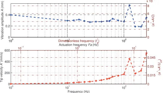
The HFVTE is designed to reach millimeter vibration amplitudes up to Fa

=

200 Hz , as shown inFig. 2. For higher

frequencies, resonance modes can be exploited to allow larger deformations. To fulfill these requirements, piezoelectric composite patches are glued on both sides of a metallic substrate. The piezoelectric components are Macro Fiber Composites (MFC) which were fabricated by Smart Material GmbH. The MFC patches are alternatively activated to provide the desired two way trailing edge displacements. Due to the substrate thickness, the patch forces create an alternate bending moment that results in the actuator vibration. To respect the airfoil shape, the assembly is covered by a silicone shell that is specifically designed to limit its impact on the actuator performance. For more information about the electro-active hybrid morphing actuators, the reader might refer toJodin et al.(2015) andScheller et al.(2016).

2.2. Experimental set up

The wing model is tested in a subsonic wind tunnel. The test section is 592 mm width per 712 mm high. The wing is mounted with an incidence of 10◦_{. As a result a blockage ratio of 18% is obtained. The blockage ratio effects are}

found to be acceptable in the present experiments which focus on the morphing effects. This is done by comparing a morphing configuration to the non-actuated case, both of which are subject to the same blockage ratio. Further explanations are introduced in Appendix C. The turbulence intensity of the inlet section is about 0

.

1% of the free stream velocity. Measurements are carried out at ambient temperature (22◦_C)._{Fig. 3}_{presents a 3D view of the wind tunnel test section}

(6)

Fig. 2. Vibration amplitude of the Higher Frequency Vibrating Trailing Edge at full voltage. The top chart presents the displacement whereas the bottom one shows the tip velocities, depending on the actuation frequency.

Fig. 3. Wind tunnel test section CAD with hybrid wing model highlighted in yellow. The PIV plane is located at mid-span and is highlighted in green. (For interpretation of the references to color in this figure legend, the reader is referred to the web version of this article.)

Smoke particles of 3

.

4

µ

m diameter are introduced in the airflow for the Time Resolved PIV (TR-PIV) measurements. The

depth of the field was focused on the stream-wise laser light sheet—inFig. 3the green area corresponds to the laser sheet within the camera range. The laser pulsations are generated by a two cavity Nd:YLF (527 nm) laser (Quantronix, Darwin Duo). The thickness of the laser sheet is 2.5 mm. Particle images are recorded during the experiment using the digital high-speed camera Phantom V1210. Each image is divided into interrogation windows. The interrogation window size is 16

×

16 px2 (px being Pixel), which corresponds to 3

.

4

×

3

.

4 mm2_{, with an overlap of 75%. The most probable displacement of the} particles between consecutive images and for a given interrogation window is obtained from the cross-correlation plane of consecutive images; DAVIS8 commercial software as well as CPIV12 _{are used for the computation. The displacement during}

the HFVTE movements reflects the resulting velocity according to the displaced trailing edge position, as the Stokes number

Sk

=

5

·

10−4_{is much smaller than one. This, as suggested by}_Green₍₁₉₉₅_{), indicates that the particles follow the motion} of the fluid. During the 45 experiments the velocity variation was below 1

.

5%. The experimental benchmark also embeds an aerodynamic balance that measures lift and drag forces. This balance is composed of two arms with strain gauges. It is worth remarking that the quantification of the lift and drag is tricky, as the measurements are significantly affected by the trailing

(7)

Fig. 4. (a) A cross section of the wing is represented with the extreme positions of the vibrating trailing edge in blue. (b) The change in effective angle of attack of the whole wing is plotted as a function of the time for different actuation cases. The effective angle of attack is defined as the angle between the straight line passing by the leading edge and the trailing edge, and the stream-wise axes. This angle depends on the camber and on the position of the vibrating trailing edge at a given time. (For interpretation of the references to color in this figure legend, the reader is referred to the web version of this article.)

edge actuator vibrations. Therefore a specific balance design as well as a detailed characterization of the sensor is performed. The balance supports the model through holes in the left and right wind tunnel test section walls. These holes are also used for connecting the morphing systems and sensors. Two small 6 mm diameter microphones and one dynamic pressure sensor (Kulite XCQ063) are implemented on the upper surface. Detailed studies have been carried out to establish the suitability of the experimental results provided in the following sections. Namely, the frequency responses of the pressure transducers are evaluated by means of calibrated white noise sound source. The characterization of the balance is carried out by evaluating the accuracy, the precision and the sensitivity to the HFVTE induced vibrations. The quality of the following statistical analysis is ensured as the time average convergence is checked, see Appendix A. The drag/lift coefficients of the current experiments are estimated within a

±

1

.

1%

/±

0

.

8% accuracy range, with a statistical confidence interval of 95%. These accuracies concern Reynolds 106_(U

∞

=

21 m

/

s) experiments. Moreover, force measurements at Reynolds 0

.

5

·

106(U∞

=

10

.

5 m

/

s) have

been carried out but do not exhibit the same accuracy and therefore are not discussed. Both Reynolds numbers experiments ensure sufficient convergence for the measurements, see Appendix B.

3. Hybrid morphing experiment overview

An experimental campaign exploring the influence of free stream velocity, angle of attack, camber, HFVTE frequency and HFVTE amplitude is performed.Fig. 1introduces the shape control range of the hybrid morphing model. To give an order of magnitude of the actuation levels of the HFVTE,Fig. 4shows the change in effective angle of attack of the wing, due to the vibrations of the trailing edge. Such a small and localized amplitude deformation is able to slightly interact with global forces on the wing. To investigate the impact of all the controlled variables, more than 3000 runs are performed. For instanceFig. 5presents the results of 476 individual measurements for different cambers, vibrations amplitudes and frequencies, at incidence of 10◦_{and Reynolds number Re}

₌

₁₀6_{. Lift coefficients are computed from balance data time} averaged on acquisitions of 20 s for camber control that displaces the trailing edge from

−

10 to +10 mm (i.e.

±

1

.

5%c) and trailing edge vibrations at frequencies from Fa

=

0–250 Hz (i.e. fa∗

=

0–8.3). The lift coefficient surface is plotted as a function

of camber and vibration frequency. Each experiment testing a HFVTE configuration is preceded by a reference measure with the same camber, the same velocity and the same incidence, but with no trailing edge vibration. This ensures the accuracy in capturing the high frequency–low amplitude actuation effects. At a given camber, the additional modifications due to the HFVTE are represented by vertical bars. The colors of these bars indicate if the HFVTE actuation increases the lift (green bars) or decreases the lift (red bars) compared to the experiment at same camber without HFVTE actuation.

A first result is the well known effect of the camber on the lift. Positively increasing the camber raises the lift, as the zero lift angle of attack shifts towards smaller values. On the one hand that up and down deformed shapes are different, leading to non-symmetrical lift effects for negative and positive cambers respectively. On the other hand characterizing the effects of trailing edge vibrations is somehow tricky. In fact, according toFig. 5, a frequency range from 100 to 250 Hz (f∗

a

∈ [

3

.

3

· · ·

8

.

3

]

) seems to be beneficial for the lift, especially for high cambers. On the other side, at low cambers the effect

of the vibration on the lift is reduced and the frequency range is shifted.

The strong coupling between the camber and the vibrating trailing edge is complex and will be the purpose of future works. As the effects of camber have already been largely assessed (see for instanceAbbott and von Doenhoff, 1949), the present work focuses on the effect of the vibrating trailing edge on the baseline cambered airfoil. To provide an insight into the vortex breakdown effect of this high frequency–low amplitude actuation, control mechanisms are described in next section. Then PIV results are detailed in the following sections. Then the results obtained in terms of local and resulting force measurements are discussed, in order to investigate the potential feasibility of a real-time on board closed loop control.

(8)

Fig. 5. (a) Modification of the measured lift coefficient Clas a function of the dimensionless camber and the dimensionless actuation frequency. The percentage lift modification is normalized to the measured lift coefficient without any morphing Cl0. (b) Corresponding 2D plots of three selected cambers. The blue areas around the data correspond to the 95% confidence level. Camber range is−10 to+10 mm and frequency range is 0–250 Hz. (For interpretation of the references to color in this figure legend, the reader is referred to the web version of this article.)

4. Wake dynamics and control mechanisms

The understanding of the operation of vortex shedding allows their control by means of morphing. The trailing edge vibration triggers eddy blocking effects that change the wake. Such changes in wake cause a vortex breakdown. The following subsections refer to results that are discussed later in this article.

4.1. Wake instability creation: Kelvin–Helmholtz instability

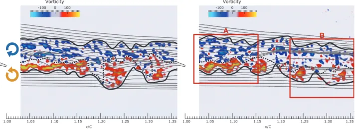
The sketch presented inFig. 6describes the mechanisms of the wake dynamics. Numerical simulations13 based on the same experimental conditions show that the detachment occurs at nearly 60% of the chord. Going downstream, this shear layer is turbulent and interacts with the Kelvin–Helmholtz vortex shedding coming from the pressure side shear layer—blue vortices in the figure. An interaction of the two shear layers coming from both sides of the wing is observed. This is also depicted by the instantaneous TR-PIV field of the non-actuated flow ofFig. 7. The trailing edge is visible on the left of the figure; the flow goes from left to right, the figure is a blow up of the wake past the trailing edge. Color shades from blue to red highlight intense vorticity areas. We clearly see a thick shear layer coming from the suction side, characterized by negative vorticity. Coming from the pressure side, a typical Kelvin–Helmholtz vortex shedding – red vortices inFig. 6 – with positive vorticity interacts and melts with the shear layer from the suction side.

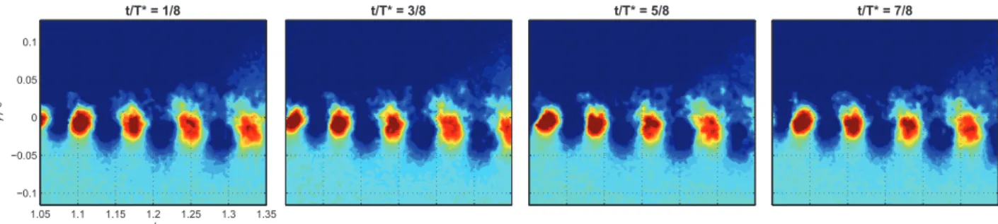
Regarding the melting of the coherent structures, it will be shown in Section6that high energy POD modes are linked to this vortex shedding (the reader can refer to mode #2 of static baselineFig. 14). This POD mode temporal coefficient spectrum exhibits a peak at a frequency St

=

11

.

5. Phase-averaged crossflow velocity component corresponding this frequency are presented inFig. 8. This clearly shows the time consistency of the vortices at this frequency over the time, as 20 periods are averaged in this figure. Finally, the spectra which will be introduced inFig. 28are computed from the crossflow velocity of 8 points in the wake. The peaks corresponding to a Strouhal of 11.5 are present everywhere. But peaks on the points corresponding to the lower shear layer are more prominent (SL peaks) and the harmonic (2SL peaks) is also present. This indicates that the Kelvin–Helmholtz instability is more present in the lower shear layer. The spectra from the upper shear layer indicate that this area is more chaotic and is dominated by the Von Kármán instability.

4.2. Wake instability creation: Von Kármán instability

In the present experimental conditions (angle of attack and velocity) the Von Kármán instability is not predominant; however the flow contains its signature and its effect. First, coherent peaks in velocity spectra fromFig. 28at a frequency

f

=

46 Hz (St

=

3

.

0) are present in the upper shear layer coming from the suction side. In the experimental study by

Huang and Lin(1995) the authors measured the Von Kármán Strouhal number (Figure 10 of the publication) as a function

of angle of attack and Reynolds number. Regarding the condition of the present paper experiment, the Strouhal is expected in the range of 0.35 by taking as characteristic length the crossflow projection of the airfoil profile. In this study, 46 Hz corresponds to a Strouhal number of 0.39 if we take the crossflow projection of the airfoil profile as characteristic length

(9)

Fig. 6. (a) Sketch of the wake dynamics. The detachment occurs at nearly 60% of the chord, shedding turbulences in the blue shear layer. Kelvin–Helmholtz instabilities appear just downstream the trailing edge; these vertical structures represented in red, coupled with those of the shear layers from the suction side, grow moving downstream. (b) Schematic representation of the eddy-blocking effect between TNT, Ref.Hunt et al.(2016). (For interpretation of the references to color in this figure legend, the reader is referred to the web version of this article.)

Fig. 7. Instantaneous PIV visualization of the static non actuated flow. The trailing edge is visible on the left of the figures; flow comes from left, the field focus on the wake just downstream the trailing edge. Color shades from blue to red highlight intense vorticity areas. (a) corresponds to the static case, (b) is for the actuation frequency f∗

a =3.7 with an amplitude of a∗ =0.04% (55 Hz, 0.3 mm peak to peak). The black lines schematically indicate the wake’s width. The mixing frontier corresponding to zero vorticity between the two shear layers (upper shear layer – blue and lower shear layer – red ) is qualitatively shown by the dashed line. (For interpretation of the references to color in this figure legend, the reader is referred to the web version of this article.)

(which still corresponds to St

=

3

.

0 when the characteristic length is the chord). This frequency is in the expected range; this is evidence of presence of the Von Kármán mode. The effect of this weak instability is described by its interaction with the Kelvin–Helmholtz previously introduced. This is explained later in the paper by the frequency named A, defined by the relation StA

=

StK−H

−

StVK.

(10)

Fig. 8. Four screenshots of crossflow component of the velocity phase average. The time period T∗_{corresponds to the frequency 172 Hz (St}₌₁₁_._{5). Here}

is the average on 20 periods.

4.3. Control strategy: from eddy blocking effect to the vortex breakdown

The eddy blocking effect has been investigated in previous studies of our research group; for example, please refer to

Hunt et al.(2016). This is qualitatively presented by the sketch inFig. 6. At a wake, a shear interface separates the turbulent region from the non-turbulent one; this interface is referred to as TNT (Turbulent–Non-Turbulent) in the following, as in the related article. The turbulent kinetic energy in the wake delimited between the two TNT interfaces is directly linked to the thickness of the shear layers, their movement and the wake’s width, i.e. the expansion or contraction of the turbulent wake. It has been shown (Hunt et al., 2008;Szubert et al., 2015)[p] that by activating smaller-scale structures of the inertial range in the turbulence energy spectrum in between the two shear layers, an upscale energy transfer is achieved towards the larger scale coherent eddies and a shear-sheltering mechanism leads to constriction of the turbulent–non-turbulent interfaces. This mechanism has been depicted in free shear layer flows (Hunt et al., 2008). Thanks to this effect, the shear layers are thinned and the distance between them is reduced. By activating higher-range POD modes where energy is concentrated in the TNT, an effect of loss of coherence on the low-range most energetic POD modes is achieved, as demonstrated bySzubert

et al.(2015). Regarding the present experiment, the eddy blocking effect can be achieved by means of morphing: by the

vibrations of the trailing edge, energy is introduced in the wake. A direct morphing-induced vortex breakdown may occur: small vortices clockwise and counter-clockwise are produced, interacting with the existing vortices of the upper and lower shear layer regions leading to pairing or breakdown of vortices depending on the sense of rotation, frequency and phase.

Fig. 7presents instantaneous PIV fields with qualitative delimitations of the shear layers. It is recalled that the leftFig. 7(a) corresponds to the baseline static case, whereas the right one7(b) corresponds to the actuation frequency f∗

a

=

3

.

7 with

an amplitude of a∗

₌

₀

_.

_{04% (55 Hz, 0}

_.

_{3 mm peak-to-peak). The turbulent wake is delimited by black lines. The interaction}

of two shear layers is schematically illustrated on the figures by black dashed lines. These two snapshots illustrate the eddy blocking effect: compared to the static baseline, the trailing edge actuation adds kinetic energy in the shear interface between the two shear layers (area A). Farther downstream, the eddy blocking effect occurs leading to a mixing and thinning of the shear layer and the wake’s width (area B). This smoothing and thinning constrain the formation of large vortices, leading to a vortex breakdown effect. As the actuation is at the trailing edge, the most affected region is the shear layer coming from the bottom side of the wing, because the flow coming from the upper side is detached.

Finally, the eddy blocking effect that shrinks the wake leads to the collapse of the coherent vortices. This causes vortex breakdown. A difference is made between these two phenomena: the eddy blocking effect consists of increasing the energy of non coherent small structures, whereas the vortex breakdown describes a decrease in energy of large coherent vortical structures.

5. TR-PIV measurements and characterization of higher frequency vibrating trailing edge effects on airflow

This section deals with TR-PIV of the wing wake, at Re

=

5

.

105_(U

∞

=

10

.

5 m/s). Results are provided and discussed for 4

test cases with baseline camber: no trailing edge vibration (static), vibrations at 55 Hz (f∗

a

=

3

.

7) at full amplitude (i.e. 1 kV

applied on actuators leading to a∗

₌

₀

_.

_{06%) and half amplitude (i.e. 500 V, a}∗

₌

₀

_.

_{03%)) respectively, and vibrations at}

12

.

5 Hz (f∗

a

=

0

.

83) at full amplitude (a∗

=

0

.

09%). The reduced frequency fa∗

=

3

.

7 is selected as it corresponds to the best

actuation from results ofScheller et al.(2015). Indeed 60 Hz has been found to be the best actuation frequency for a 0

.

42 m chord wing section with NACA 4412 airfoil and free stream velocity of 7 m/s. The dimensionless actuation frequency in this work is evaluated as f∗

a

=

3

.

7. On the other hand 12

.

5 Hz is selected as it is a low mechanical resonance of the actuator—which

does not excite the whole wing structure. Therefore, this low actuation frequency with its harmonics provides magnitudes large enough to affect strongly the dynamics of the flow as will be shown in the following results.

This section focuses on experiments at Reynolds number of 5

·

105, whereas the force measurements presented in the last section are performed at Reynolds number of 106_{. This is due to technical limitations. Performing TR-PIV at high Reynolds} numbers requires large acquisition frequencies. As the memory of the high speed camera is limited, experiment record durations are inversely proportional to Reynolds number. Specifically for Re

=

5

·

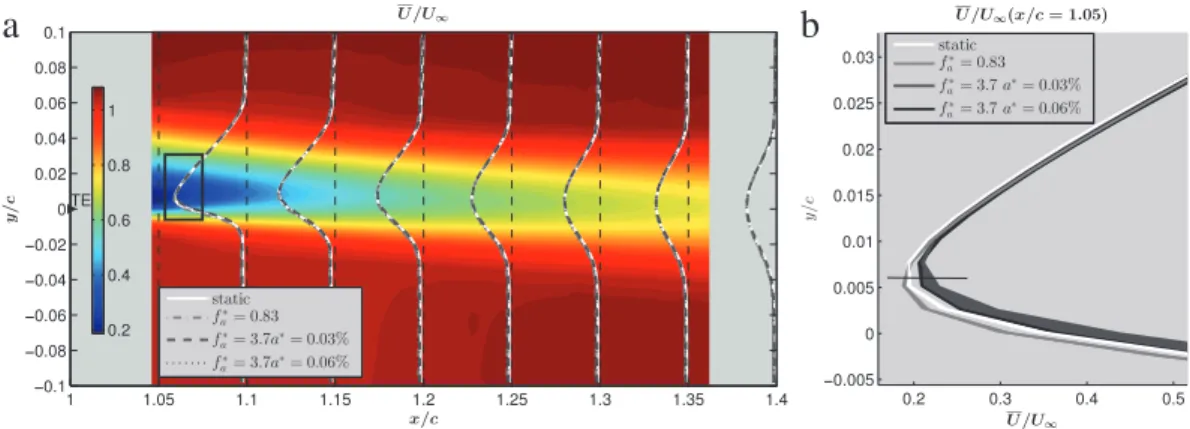
105_{the acquisitions last more than 11 s.}

(11)

Fig. 9. Time average of the stream-wise velocity component for the static case and velocity profiles for the non-actuated and the actuated configurations; Re=0.5·106_{. The thicknesses of the envelopes corresponds to minimum and maximum values calculated using the three acquisitions. (For interpretation} of the references to color in this figure legend, the reader is referred to the web version of this article.)

Fig. 10. Time average of the squared stream-wise perturbation velocity u2 _{for the static case and profiles for the non-actuated and the actuated} configurations; Re=0.5·106_{. The thicknesses of the envelopes corresponds to minimum and maximum values calculated using the three acquisitions.}

On the other hand for Re

=

106experiment records are only 6

.

5 s. The physical PIV interpretations provided in the following concern experiments at Reynolds number of 5

·

105_.

Time averages of the velocity fields are computed from the TR-PIV for the different configurations.Fig. 9on left presents the contour plot of time average stream-wise velocity for the static experiment. Black and gray vertical lines represent cut lines corresponding to the superimposed velocity profiles of experiments. Namely velocity profiles are extracted for x

/

c

equal to 1.05, 1.10, 1.15, 1.20, 1.25, 1.30 and 1.35. The values of each curve are normed so that the maximum value among each set of curves does not cross over the neighboring sets, i.e. within a

±

0

.

05 horizontal unit. This figure should allow the reader to compare the evolution of the wakes for the different test cases. The experimental results appear close to each other, so the velocity profiles at x

/

c

=

1

.

05 corresponding to the black box on the left plot are represented on the right of the figure. Namely, for each of the 4 test cases 3 acquisition runs are performed to check the repeatability of the measurements. The lines represent the average velocity profiles within envelopes of the same color tones corresponding to the maximum and minimum measurements. Compared to the static case, actuating at f∗

a

=

0

.

83 (12

.

5 Hz) increases the velocity defect. On the

other hand forcing at f∗

a

=

3

.

7 (55 Hz) – with amplitudes of both a∗

=

0

.

06% (1000 V) and a∗

=

0

.

03% (500 V) – slightly

decreases the wake thickness, with consequent potential benefits in terms of drag reduction. These two actuations decrease the velocity defect by more than 3% in average, as visible inFig. 9(b).

Differences between experiments are more clearly visible inFig. 10, which represents the energy of the fluctuating stream-wise component of Reynolds stress tensor u2_{. Consistently with}_{Fig. 9}_{, the left plot displays the mean stress tensor} field for the non actuated configuration. The u2_{profiles corresponding to the different test cases are superimposed. The right} plot is a zoom on u2_{profiles at x}

_/

_c

₌

₁

_.

_{20. The turbulent energy associated to the Reynolds stress u}2_{appears concentrated} in two regions of the wake: the most energetic one is just past the trailing edge, whereas the second one is located above the trailing edge, coming from the wing suction side.

It appears that actuation concentrates the energy in the shear layer, leading to an increase of u2_{in the lower region of the} wake, whilst decreasing the energy of the upper area. Actuating at f∗

a

=

3

.

7

,

a∗

=

0

.

03% (55 Hz, 500 V) decreases u2in both

upper and the lower parts of the wake.

Fig. 11shows the

v

2_{Reynolds stress. The effects of actuation on this component are more significant. The peaks of this} quantity are located in the lower part of the shear layer. Namely actuation at f∗

(12)

Fig. 11. Time average of the squared crossflow perturbation velocityv2_{for the static case and profiles for the non-actuated and the actuated configurations;} Re=0.5·106_{. The thicknesses of the envelopes corresponds to minimum and maximum values calculated using the three acquisitions.}

Fig. 12. Time average of the turbulent kinetic energy u2₊_v2_{; Re = 0}_.₅_·₁₀6_{. The thicknesses of the envelopes corresponds to minimum and maximum} values calculated using the three acquisitions.

peak, whereas actuation at f∗

a

=

3

.

7 (55 Hz) increases it by up to 10%. It also appears that all of the actuated configurations

reduce the

v

2_{stress component just behind the trailing edge (at x}

_/

_c

₌

₁

_.

_05).

Fig. 12displays the flow field and the profiles of the quantity u2

₊

_v

2_{. Reasonably assuming the flow as incompressible,}

u2

₊

_v

2_{may be considered as a representation of the turbulent kinetic energy.} Actuating at f∗

a

=

3

.

7 (55 Hz) decreases the energy just past the trailing edge (x

/

c

=

1

.

05). The opposite is obtained

when actuating at f∗

a

=

0

.

83 (12

.

5 Hz). Moving downstream, the wake forced at fa∗

=

0

.

83 (12

.

5 Hz) exhibits a significant

decrease in kinetic energy on the lower area. On the other side a light decrease in kinetic energy is observed on the upper part of the wake (flow coming from the suction side). Actuating at 55 Hz and 1000 V slightly decreases the turbulent kinetic energy. On the contrary the actuation at 55 Hz and 500 V seems to increase the flow energy.

Overall the best actuation in terms of turbulent kinetic energy seems to be at a frequency of 12

.

5 Hz. The energy is concentrated close to the trailing edge, and it quickly decreases moving downstream. Actuation at f∗

a

=

3

.

7 a∗

=

0

.

06%

(55 Hz 1000 V) seems to have no significant effect on kinetic energy. Finally for f∗

a

=

3

.

7 a∗

=

0

.

03% (55 Hz 500 V) actuation

appears to essentially increase the wake energy.

6. Proper orthogonal decomposition of the wake flow

In order to have a better understanding of the flow behavior, a proper orthogonal decomposition (POD) is performed on the measured velocity field for the tests at Re

=

0

.

5

·

106and angle of attack of 10◦_{. The POD has been computed on the entire}

PIV field. The vorticity of each mode is also computed. The POD allows for detecting the coherent structures featured by the flow field on the basis of their wake number and frequency. The POD is extensively used for the assessment of turbulent flow fields, when dealing with experimental data, or with numerical computations (Berkooz et al., 2011).

(13)

The velocity field can be expressed as a composition of spatial and temporal modes as follows: U′ (x

,

t)

=

n

X

i=1

φ

i(x)ai(t)

,

(1)

being

φ

i(x) and ai(t) the ith spatial and temporal modes, respectively. The method proposed inPerrin(2005) is selected

among the several techniques employed for the flow modal decomposition. This approach is particularly suitable for experimental data. As the field is discretized in Nxspatial samples for each N snapshots, PIV issues a matrix of data that

can be written as:

M

=







u1 1 u 2 1 u N−1 1 u N 1 u1 2 u 2 2 u N−1 2 u N 2 u1 Nx u 2 Nx u N−1 Nx u N Nx

v

₁1

v

2₁

v

₁N−1

v

N₁

v

₂1

v

2₂

v

₂N−1

v

N₂

v

_N1_x

v

2_N_x

v

_NN_x−1

v

_NN_x







.

(2)

The correlation matrix required for the modal decomposition is computed as :

R

=

1

NM

T

_·

_M

_,

₍₃₎

and the corresponding eigenvalue problem writes

RA

=

λ

A

,

(4)

being

λ

the array of eigenvalues and A the matrix of eigenvectors. The computed eigenvalues are then rearranged in descending order as

λ

1

> λ

2

> · · · > λ

N

=

0. The matrix of eigenvectors is employed to compute the spatial modes

as follows:

φ

i

=

P

N j=1Aijuj

P

N j=1A i juj

,

i

=

1

,

2

, . . . ,

N (5)

being

φ

ithe ith spatial mode. The computation of the temporal modes is straightforward:

ai

=

φ

iM

.

(6)

Based on 15 000 snapshots, the first 200 modes are retained from the POD. In the following only the first five modes and the higher order modes exhibiting the most significant vortical structures are displayed and discussed in a first time. Section6.5deals with higher POD modes to underline the control strategy. Namely, Von Kármán, Kelvin–Helmholtz and two other coherent vortical structures have been detected within the wake. First the static configuration, i.e. with the trailing edge non-actuated, is discussed. Then PODs for the velocity fields obtained by trailing edge actuation at frequency f∗

a

=

3

.

7

(55 Hz) and amplitude a∗

₌

₀

_.

_{03% (500 V) and a}∗

₌

₀

_.

_{06% (1000 V) respectively are illustrated. Finally the spatial and}

temporal modes for excitation at frequency f∗

a

=

0

.

83 12

.

5 Hz and amplitude a∗

=

0

.

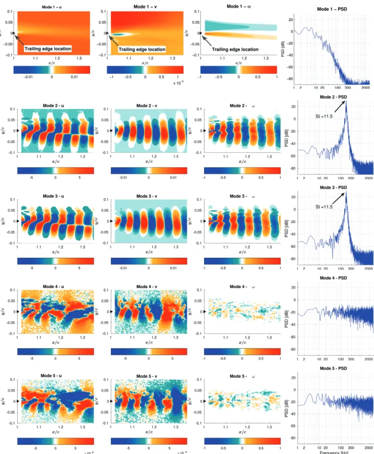
09% (1000 V) are described.

TheFigs. 14,16,18,20,21,22a,23,24,27,26represent from left to right: (i) the stream-wise component of the ith spatial velocity mode; (ii) the crossflow component of the ith spatial velocity mode; (iii) the vorticity computed for the corresponding ith spatial velocity mode; (iv) the power spectral density (PSD) of the temporal mode associated to the velocity magnitude. The velocity spatial modes are normalized by the free stream velocity. The black triangle on the left hand side of the flow fields represents the location of the wing trailing edge.

The PSDs are computed using the Welch’s weighted overlapped segment averaging estimator (Welch, 1967). Periodogram estimations use 4 s Hamming windows with 64% overlap (minimum variance) and zero padding. The shedding frequencies are often provided in non dimensional form, using Strouhal number.

6.1. POD of the PIV measurements for the baseline configuration

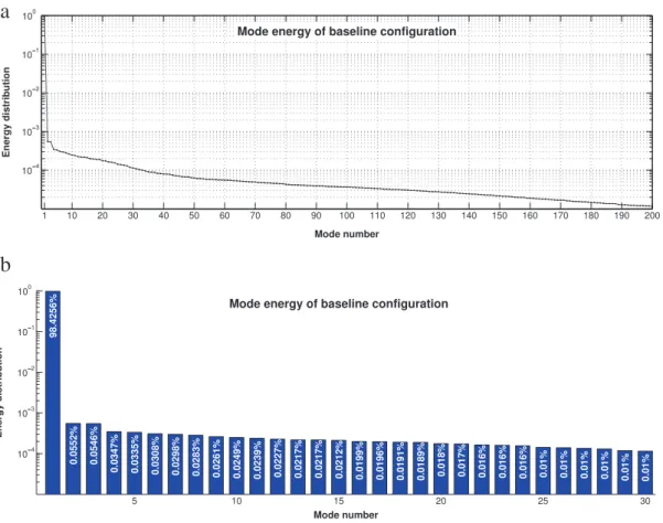
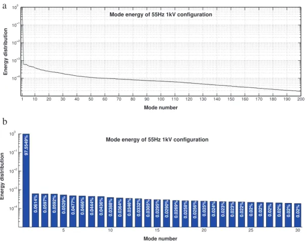
Fig. 14displays the first five modes issued by the POD. The first mode (four plots on the top of the figure) corresponds to the time average of the flow field. The wake region is clearly visible both on the velocity and on the vorticity fields. In particular the two counter-rotating vorticity regions correlated to the flow from the upper and on the lower side of the wing section are clearly visible. The PSD of the temporal mode decays rapidly, as expected for the mean field. The energy content of mode #1 is equal to the 98

.

4% of the total energy, seeFig. 13. An estimation of the energy featured by a specific mode is provided by the associated eigenvalue, or equivalently by the area subtended by the PSD of the temporal mode. Modes #2 and #3 exhibit shear layer vortical structures, detectable both on the velocity and on the vorticity fields. The peak at

(14)

Fig. 13. Energy distribution of the first modes issued from the POD for the baseline configuration. The first 200 are presented in (a), (b) focuses on the first 30.

Strouhal St

=

11

.

5 observed in the PSD confirms shedding phenomena typical of Kelvin–Helmholtz instabilities. The shear layer instability frequency is consistent with the estimation provided in Section4, as well as with the findings ofSzubert et al.(2015) for numerical simulations in transonic conditions. With this regard it is worth remarking that the flow beside the wake inSzubert et al.(2015) features local Reynolds number comparable to that of the experiments carried out in the present work. In fact the flow is substantially decelerated downstream the shock on the suction side. By considering at the velocity fields of modes #2 and #3, they are in space quadrature, and additionally they feature the same spectrum and the same energy content. Therefore a progressive wave of counter-rotating vortices occurs, alternately shed from the trailing edge, and convected downstream.

Modes #4 and #5 seem chaotic and are discussed in6.5.

6.2. POD of the PIV measurements for HFVTE at f∗

a

=

3

.

7 a∗

=

0

.

03% (55 Hz 500 V)

Results of the POD performed for the velocity data measured with actuation at f∗

a

=

3

.

7 a∗

=

0

.

03% (55 Hz and amplitude

500 V) are discussed here. The trailing edge tip cross flow peak to peak velocity imposed by the actuation corresponds to 1%U∞. The reader can refer toFig. 2(performance of the HFVTE actuator), assuming in this actuation case the vibration

amplitudes and velocities are halved, as the voltage is halved compared to the 1 kV characterization in the figure (specifically, assuming linear piezoelectricity).

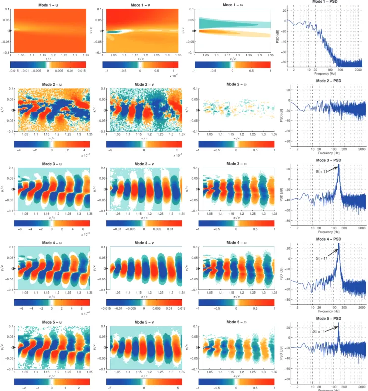
Fig. 16shows the first five spatial modes, together with the PSD of the corresponding temporal mode. The first row of

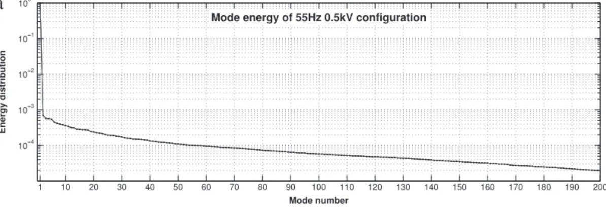
figures from the top is the first mode, therefore it describes the mean behavior of the wake. The velocity and vorticity fields, as well as the PSD of the temporal mode, resemble the static counterpart. However in this case the energy associated to the first mode contains the 97

.

5% of the total energy, therefore it is smaller than the static analogue. As a consequence a larger fraction of energy is contained within the higher order modes, seeFig. 15.

The second row of plots inFig. 16displays the second mode of the POD. Mode #2 shows non-coherent vortices with almost flat and high amplitude PSD. Modes #3 and #4 exhibit Kelvin–Helmholtz vortices. Their frequency shifts from St

=

11

.

5 (173 Hz) of the non-actuated case, to St

=

11 (165 Hz). The corresponding dimensional frequency of 165 Hz corresponds to three times the actuation frequency. Mechanisms of such change in flow due to morphing are explained in Section6.5.

(15)

Fig. 14. POD of the first five modes for the non actuated configuration. From left to right: stream-wise velocity component; crossflow velocity component; vorticity of the corresponding mode; PSD of the temporal coefficients of each POD mode.

a

=

3

.

7 a∗

=

0

.

06% (55 Hz 1000 V)

Fig. 18shows the first five POD modes extracted by the measured velocity field. The energy content of the first mode is

(16)

Fig. 15. Energy distribution of the first modes issued from the POD with trailing edge harmonic actuation at f∗

a =3.7 a∗=0.03% (55 Hz 500 V). The first 200 are presented in (a), (b) focuses on the first 30.

when doubling the actuation amplitude, as shown inFig. 17. Mode #2 exhibits a tight peak in the PSD of the temporal mode at three times the actuation frequency, i.e., St

=

11. This mode is associated with coherent vortical structures not observed within the non actuated configuration. The energy content of mode #2 is found to be larger compared to the static counterpart.

With regard to modes #3 and #4 similar effects to those obtained when actuating at 500 V are observed. Namely Kelvin– Helmholtz structures are shifted to St

=

11 (165 Hz), corresponding to three times the actuation frequency. The mechanisms of such change in flow due to morphing are explained in Section6.5.

a

=

0

.

83 a∗

=

0

.

09% (12

.

5 Hz 1000 V)

The response of the flow to harmonic excitations at frequency f∗

a

=

0

.

83 (12

.

5 Hz) and amplitude a∗

=

0

.

09% (1000 V)

is finally investigated by means of POD. The deflection velocity of the trailing edge tip is 0

.

45%U∞.

Fig. 20shows the first five modes issued by the POD of the measured velocity field. The first mode, corresponding to the time average of the velocity and of the resulting vorticity, features an energy content of 97

.

6%, not dissimilar to that of the static counterpart, seeFig. 19.

The energy content of mode #2 contains the 0

.

06% of the total energy amount. The corresponding velocity and vorticity fields show non-coherent vortices with almost flat and high amplitude power spectral density. The flow energy of this mode appears to be significantly increased compared to the non-actuated case. A similar phenomenon as f∗

a

=

3

.

7 a∗

=

0

.

06%

(55 Hz 500 V), i.e. a new chaotic second POD mode is found. Discussion is detailed in Section6.5.

The PSD of mode #3, #4 and #5 show peaks at 10 times the actuation frequency (St

=

8

.

5), associated to very coherent structures and corresponding to Kelvin–Helmholtz vortices. Moreover, a secondary energy peak is visible at St

=

11

.

7 (175 Hz), i.e., 14 times the actuation frequency.

6.5. Wake mechanisms, higher order modes and control strategies

This section now details some wake mechanisms and focuses on comparison between the different actuations. The control strategy described in Section4is illustrated with experimental results.

(1) Von Kármán vortex shedding. Regarding the static baseline, two coherent structures are also observed at St

=

8

.

5 (127 Hz) and at St

=

3 (46 Hz), or multiples of this latter frequency.Fig. 21shows an example of a mode where coherent

(17)

Fig. 16. POD of the first five modes with trailing edge harmonic actuation at f∗

a =3.7 a∗=0.03% (55 Hz 500 V). From left to right: stream-wise velocity component; crossflow velocity component; vorticity of the corresponding mode; PSD of the temporal coefficients of each POD mode.

structures at these frequencies are detected. Specifically modes where peaks at multiples of St

=

3 (46 Hz) are detected are #8, #9, #16, #17, #18, #19, #20, #24, #27, #34 and #35. Modes with vortex shedding phenomena at St

=

8

.

5 (127 Hz) are #12, #13 (Fig. 23), #14, #15, #16, #17, #18, #19, #21, #22, and #24. As a consequence, there are some modes which exhibit both of these two vortical structures, respectively coupled, seeFig. 21. It is worth noting that this coupling is found to be strongly affected by the trailing edge actuation discussed in the following. The peak at St

=

3 (46 Hz) can be associated with the Von Kármán instabilities. The peak at 127 Hz (which will be referred to as the letter A in the next section) is a combination of Von Kármán (VK) and shear layer (SL) instabilities according to: StA

=

StSL

−

StVK.

(2) Higher order mode St

=

14.Fig. 22ashows the mode #36 issued by the POD of the static case. This mode shows a special coherence and the PSD for the temporal mode corresponds to St

=

14

.

1 (212 Hz peaks referred to as B in Section5). The corresponding modes in case of morphing at f∗

(18)

a =3.7 a∗=0.06% (55 Hz 1000 V). The first 200 are presented in (a), (b) focuses on the first 30.

inserts new patterns. For this reason, in the morphing case, mode #39 of the actuated case is compared to mode #36 of the static case (seeFig. 22b). It can be seen that this mode has lost its spatial coherence, the spectrum does no more display predominant peaks and the vorticity field of this mode indicates a significant of the wake thickness, corresponding to approximatively 15%. This morphing induced effect is analogue to the re-injection of turbulence by means of higher-order POD modes studied numerically bySzubert et al.(2015), enhancing an eddy-blocking effect.

It is also worth remarking that none of the 60 modes retained from the POD for all actuation cases exhibit peaks at St

=

14

.

1 (212 Hz). This confirms that these coherent structures are actually dissipated and are not moved towards larger wave numbers. This is an example of vortex breakdown.

(3) Shift of modes associated to the shear layer towards higher order-lower energy modes. Both actuations at

f∗

a

=

3

.

7 a∗

=

0

.

03% (55 Hz, 500 V) and fa∗

=

0

.

83 a∗

=

0

.

09% (12

.

5 Hz, 1000 V) exhibit a downshift of the modes #2

and #3 compared to the static baseline. This effect is also present on the f∗

a

=

3

.

7 a∗

=

0

.

06% (55 Hz, 1000 V) with a higher

presence of the actuation frequency in the spectra, due to a larger forcing amplitude. The cause is twofold.

Firstly, the forced flow is found to exhibit vortex shedding phenomena at super-harmonics of the actuation frequency. The two actuations at f∗

a

=

3

.

7 (55 Hz) have shifted the Kelvin–Helmholtz shedding frequency from St

=

11

.

5 to 3 times the

actuation frequency St

=

11

=

3

·

f_a∗. Actuation at f∗

a

=

0

.

83 has shifted this frequency to 10 times the actuation frequency St

=

8

.

5

=

10

·

f_a∗. Again the forced flow is found to exhibit vortex shedding phenomena at super-harmonics of the actuation frequency. A similar behavior was showed for instance inMotta and Quaranta(2015) andMotta(2015) on the flow response to a harmonically oscillating L-shaped Gurney flap.

Secondly, morphing introduces a new chaotic second mode—see modes #2 inFigs. 16and20. This energy injection is the signature of the eddy blocking effect described in Section4. The modes #3 and #4 of the morphing case are similar to the modes #2 and #3 of the baseline, so morphing causes the shift of these two modes to higher order. These two modes characterize the main vortex shedding of the wake lost energy. This downshift in energy is associated to vortex breakdown. Specifically, the energy distribution of this morphing case (f∗

a

=

3

.

7 a∗

=

0

.

03%) shows that the chaotic mode #2 is 3% more

energetic than the coherent mode #3—seeFig. 15. This decrease in energy reaches the value of 23% between mode #2 and #3 for the f∗

a

=

0

.

83 a∗

=

0

.

09% morphing case—seeFig. 19. Further shifts in the flow modes with respect to the static case

are observed when actuating at f∗

a

=

3

.

7 a∗

=

0

.

03% (55 Hz, 500 V). Namely coherent structures observed for mode #16 of

the static configuration are found on mode #32, not reported here for brevity purposes.

(4) Shear layer thinning. Morphing effects on wake thickness are visible on higher POD modes. For instance, the mode

#13 of the static baseline (Fig. 23) indicates wake expansion. The actuated case at frequency f∗

(19)

1000 V) illustrates the eddy blocking effect. The POD mode #22 (Fig. 24) corresponds to the baseline mode #13, because there are similarities in the spatial mode distribution and their temporal coefficients show the same peak at Strouhal of 8.5; besides, actuation frequency is present in the spectrum of the morphing case (Fig. 24(d)). The

v

component of the mode indicates a thinner wake which decreases in the wake expansion, after x

/

c

=

1

.

25. The wake thickness, indicated by arrows on Figs.23(c),24(c) is reduced by approximately 22% at x

/

c

=

1

.

35, thanks to the actuation. One can also remark that – due to the morphing – the magnitude of the characteristic peak at Strouhal of 8.5 has decreased by 10 dB, which means the power density divided by 10.

(5) Downshift of the higher energy chaotic modes. Now considering the modes #4 and #5 of the static baseline (Fig. 14

orFig. 25), similarities can be found with modes #57 of the case f∗

a

=

3

.

7

−

a∗

=

0

.

03% (Fig. 26) and the mode #40 of the case f∗

(20)

a =0.83 a∗=0.09% (12.5 Hz 1000 V). The first 200 are presented in (a), (b) focuses on the first 30.

are chaotic but with high energy. The corresponding morphing modes have thinner wakes, due to the eddy blocking effect. Spectra of morphing modes #40 and #57 present peaks that are not present in the static modes; these peaks correspond to harmonic of the actuation frequencies: the Strouhal of 9.2 corresponds to 11 times the actuation frequency (9

.

2

≃

11

·

0

.

83) for the mode #40 whereas the Strouhal of 11 corresponds to 3 times the actuation frequency for the mode #57 (11

≃

3

·

3

.

7). It is worth noting that these two morphing cases, both different in amplitude and frequency generate equivalent effects.

6.6. General remarks on the POD results

The proper orthogonal decomposition is carried out on the wake velocity field measured by PIV surveys. The first 60 modes issued by POD are investigated in terms of velocity and vorticity fields. The PSD of the temporal mode is also analyzed. It appears that the vortical structures observed at certain frequencies on the unforced flow are shifted to the actuation frequencies or to their higher harmonics. This effect occurs equally for the two actuation amplitudes here considered. With this regard it appears that for the excitation frequency of f∗

a

=

3

.

7 (55 Hz), actuating at a∗

=

0

.

03% (500 V) is more

favorable compared to a∗

₌

₀

_.

_{06% (1000 V), where a significant increase in the energy of mode #2 relative to the static}

case is observed. In general comparing the unforced and the forced flow, this latter features a slightly higher level of energy. The fact that the same vortical structures are observed on higher order modes relative to the static case is an indication that a proper vortex breakdown – limited to the larger coherent structures – is occurring. The turbulent fluctuation dynamics shows significant modifications due to the morphing:

•

shift of the non-actuated modes 2 and 3 (Fig. 14) associated to Kelvin–Helmholtz towards the higher order modes 4 and 5 (Fig. 20) for actuated case;

•

disappearance of coherent higher frequency modes: St

=

14 for instance, shift of modes associated to the shear layer towards higher-order lower-energy modes ;

•

shear layer thinning at x

/

c

=

1

.

35 of order 22% (Figs.23(c) and24(c)) ; and

•

decrease of spectral amplitude of the peak at St = 8.5, Figs.23(d) and24(d).

Furthermore, the flow response to wake forcing is similar to that reported inSzubert et al.(2015) for transonic flow conditions. This confirms the potential suitability of high frequency actuation both for subsonic flow conditions here investigated typical of descent flight, and for cruise speeds.

(21)

a =0.83 a∗ =0.09% (12.5 Hz 1000 V). From left to right: stream-wise velocity component; crossflow velocity component; vorticity of the corresponding mode; PSD of the temporal coefficients of each POD mode.

7. Spectral analysis of flow velocity

The crossflow velocity component is extracted for 8 points from the TR-PIV measurements. These points are located in the wake close to the trailing edge and downstream, below and above the trailing edge. The center ofFig. 28presents the time average stream-wise velocity field of the non-activated baseline flow. The 8 points are numbered on the field. The trailing edge is visible on the left. The different Power Spectral Densities (PSD) of the crossflow velocities are presented in the spectra around the central velocity field. The PSDs are again computed using the Welch’s weighted overlapped segment averaging estimator (Welch, 1967). To maximize the accuracy of the estimator, temporal signals of the three experiment repetitions are concatenated to obtain 33 s signals. Periodogram estimations use 4 s Hamming windows with 64% overlap (minimum variance) and zero padding.

(22)

Fig. 21. POD mode #16 for the non actuated baseline configuration. From left to right: stream-wise velocity component; crossflow velocity component; vorticity of the corresponding mode; PSD of the temporal coefficients of each POD mode.

(a) Mode #36 for the non-actuated baseline.

(b) Mode #39 for the f∗

a =3.7 a∗=0.03% morphing case.

Fig. 22. Comparison of two POD modes. From left to right: stream-wise velocity component; crossflow velocity component; vorticity of the corresponding mode; PSD of the temporal coefficients of each POD mode.

Fig. 23. POD mode #13 for the non actuated baseline configuration. From left to right: stream-wise velocity component; crossflow velocity component; vorticity of the corresponding mode; PSD of the temporal coefficients of each POD mode.

According to the POD results, the flow energy is mainly dominated by the shear layer (SL) coherent instabilities. This corresponds to the SL arrows pointing to the frequency peaks. The shear layer instability is more concentrated in the lower flow, as the SL peaks of points 1 to 4 are over

−

130 dB and the second harmonics are visible (2SL peaks). The points 1, 2, 5 and 6 which are located close to the trailing edge show the frequency signature of the Von Kármán vortices—presented by VK and VK/2 arrows. Coherent structures highlighted by POD analysis at Strouhal of 14.1 appear as B peaks. These peaks are absent from points 6 and 8 corresponding to the flow coming from the suction side. The Von Kármán Strouhal number is evaluated to 3. This is again comparable to CFD simulations ofSzubert et al.(2015) with a Strouhal of 2.4 (computed relatively to the

(23)

Fig. 24. POD of mode #22 with trailing edge harmonic actuation at f∗

Fig. 25. POD of mode #5 for the non actuated baseline configuration. From left to right: stream-wise velocity component; crossflow velocity component; vorticity of the corresponding mode; PSD of the temporal coefficients of each POD mode.

Fig. 26. POD of mode #57 with trailing edge harmonic actuation at 55 Hz and 500 V. From left to right: stream-wise velocity component; crossflow velocity component; vorticity of the corresponding mode; PSD of the temporal mode for the velocity magnitude.

Fig. 27. POD of mode #40 with trailing edge harmonic actuation at 12.5 Hz and 1000 V. From left to right: stream-wise velocity component; crossflow velocity component; vorticity of the corresponding mode; PSD of the temporal mode for the velocity magnitude.

chord with the frequency 2630 Hz). Peaks A, present on each of the considered points, correspond to the coupling of the Von Kármán and the shear layer structures. Indeed the Strouhal of the peak A is linked to these structures by the relation

StA

=

StSL

−

StVK. Physically, this can be interpreted as Kelvin–Helmholtz amplitude modulation due to the Von Kármán

instabilities. This peak identification not only allows for the understanding of the phenomena but also allows identifying spectral signatures in the flow. These signatures can be detected by pressure transducers (see Section8). In addition, the flow is significantly affected by the actuation and its effects are clearly visible on the reported spectra.

(24)

Fig. 28. PSD of the crossflow velocity on the 8 extracted points, from the baseline configuration. The center figure presents the positions of the extracted points within the time average stream-wise velocity.

The crossflow velocity component is extracted for the actuated configurations. Globally the peaks described above are still visible, but some modifications are noticeable. As some spectra are similar, only signals from points 4, 5 and 8 are compared.

Fig. 29shows a comparison in PSD of point 4 between the baseline and the f∗

a

=

0

.

83 (12

.

5 Hz) actuation. The frequency

range is focused on Strouhal from 7.5 to 15. Actuation harmonic frequencies from 9 to 18 are presented on the x-axis. Peaks of baseline flow named A, SL and B are withdrawn by the actuation. In exchange the actuation gives rise to other peaks. Most of them have lower amplitude and others are harmonics of the actuation frequency. Black arrows indicate peaks corresponding to harmonics of the actuated flow. This phenomenon tends to spread the peak energies over actuation harmonics and over other frequencies. This could be interpreted as a vortex breakdown of the largest coherent structures.

Concerning the other points in the wake and the other actuation cases,Table 1deals with the Root Mean Square (RMS) values of fluctuating crossflow velocity

v

2_{of the 8 extracted points. Variations compared to the non actuated baseline are} calculated in percentage. The turbulent energy is decreased by 5% to 7% everywhere for the f∗

a

=

0

.

83 (12

.

5 Hz) actuation. The f∗