OATAO is an open access repository that collects the work of Toulouse
researchers and makes it freely available over the web where possible
Any correspondence concerning this service should be sent
to the repository administrator:
[email protected]
This is an author’s version published in: http://oatao.univ-toulouse.fr/21621
To cite this version:
Míguez, J. M. and Piñeiro, M. M. and Algaba, J. and Mendiboure, B. and Torré,
Jean-Philippe
and Blas, F. J. Understanding the Phase Behavior of Tetrahydrofuran + Carbon
Dioxide, + Methane, and + Water Binary Mixtures from the SAFT-VR Approach. (2015) The
Journal of Physical Chemistry B, 119 (44). 14288-14302. ISSN 1520-6106
Official URL:
https://doi.org/10.1021/acs.jpcb.5b07845
properties and the full THF + water phase diagram can be found elsewhere in literature.3,4
THF is a powerful gas hydrate promoter, as it follows forming mixed gas hydrates (i.e., hydrates containing both THF and another guest gas, such as THF + CO2hydrate) at lower pressure and higher temperature than the hydrate formed without this promoter (the CO2hydrate in that case).5,6This property has been widely exploited to produce hydrates in appropriate temperature and pressure ranges depending on the application envisaged. As an example, several authors7−9 used THF to significantly reduce the equilibrium pressure of H2 clathrate hydrate, considering its application in H2storage cells. The effect on the phase equilibria was clear, although as pointed out by Struzhkin et al.,10 some issues remain concerning, for instance, the distribution of both guest molecules between both types of cells within the sII structure. Nevertheless, the role of THF in H2storage using hydrates is clear, as pointed out recently in the review of Veluswamy et al.11
The same effect has been pointed out for carbon dioxide (CO2) hydrates, and the environmental concern related with greenhouse gas emission control and the effects on global climate change have attracted intense research efforts in this direction. Kang and Lee12 showed the thermodynamic feasibility of using THF to tune hydrate phase equilibria in the process of recovering CO2 from postcombustion or industrial flue gases. This topic is very active right now and many recent works13−15continue studying different aspects of this process.
The cornerstone of these applications is the multiphasic equilibria of THF mixtures, and if from an experimental perspective the number of studies published is very large, from a molecular modeling perspective the subject is undoubtedly far behind in development. Considering for instance the latest application cited, CO2 capture using hydrates, a proper theoretical description of the process entails at afirst stage an accurate description of phase equilibria of fluid solutions containing at least THF, CO2, and water (H2O). This is a complicated task, and although many attempts have been devoted to describe these complex phase equilibria scenarios, the discussion is still open. In any case, the complexity of an accurate description of aqueous solutions phase equilibria is well known, and even if binary mixtures are sometimes well described, the effects in multicomponent mixtures are poorly understood.16
The characteristics of THF make it a remarkably difficult target for molecular modeling. This is due to its cyclic structure, and the presence of the ether group, which produces a strong polarity, and a marked spacial anisotropy, inducing complex intermolecular interactions with the possibility of hydrogen bonding. Determining the degree of detail of a molecular model to represent this molecule with a physically realistic representation and accurate results without falling in over parametrization is a challenging objective. Avoiding an excessive degree of dependence between results and parametrization and seeking for parameter transferability are desirable objectives that should also be kept in mind. This applies to different levels of calculation, from equations of state (EoS) modeling to molecular simulation. Setting the proper molecular model is the first step toward a reliable representation of phase equilibria, and this should include first a robust representation of fluid phases before considering solid−fluid equilibrium, where hydrate description lays at the very end of this path. Another
point in this discussion is the interest of defining molecular models that can be used with exactly the same definition, structural details, and characteristic parameters in the frame work of different approaches as EoS and molecular simulation,17 to obtain the best from each scheme. This includes the ability of EoS to describe phase equilibria and thermodynamic properties over broad temperature and pressure ranges with short calculation times, combined with the possibility of studying in detail microscopic fluid features with molecular simulation.
In this context, the description of THF has been attempted using different approaches and proposing different molecular models. A representative example of this is the recent work by Herslund et al.,18where different models are proposed for THF in the framework of CPA19 EoS, discussing the degree of molecular detail in the description of phase equilibria of its aqueous solutions. The authors show how deciding a priori the association bonding scheme for the molecular models determines its performance for this highly nonideal solution. Let us recall that this binary global phase diagram can be ascribed as type VI according to van Konynenburg and Scott20,21 classification, and accordingly, it presents the distinctive feature of a closed loop miscibility gap at moderate pressures, which has been accurately described experimen tally.22−24From a theoretical point of view, this behavior is a challenge and a major benchmark for any molecular modeling attempt.
Giner et al.25 studied the phase equilibria of pure cyclic ethers using the SAFT VR molecular EoS. This EoS considers the molecules formed by tangentially bonded variable range square well (SW) segments, with specific additional interaction sites to account for associating interactions. In the cited work,25 cyclic ethers were considered as nonassociating, and polar effects were neither considered. The parameters determined were later used to estimate vapor liquid equilibria of mixtures with chloroalkanes,26,27 obtaining fairly good results. This modeling approach is the same used in one of our previous works16 to study the global phase diagram of the binaries including H2O, CO2, and methane (CH4), and their ternary mixture. In that case, SAFT VR EoS proved to be able to describe a very complex phase equilibria scenario resulting from the combination of type I and type III binary mixtures, using pure component parameters determined previously by other authors and used, in this case, in a completely transferable manner, needing only one additional binary mixing rule coefficient for the H2O + CO2 binary. These results have induced us to apply the same approach for the estimation of THF solutions phase equilibria, considering its mixtures with the same three molecules, H2O, CO2, and CH4, for the interest they have toward the understanding of hydrates phase equilibria. As it will be shown later, this implies describing type I, THF(1) + CO2(2), type III, THF(1) + CH4(2), and type VI, THF(1) + H2O(2) binary phase diagrams with the same set of transferable molecular parameters.
■
MOLECULAR MODELS AND THEORYSAFT-VR Molecular Models. SAFT VR approach requires the determination of a number of intermolecular parameters to describe the thermodynamic phase behavior of real substances. In this EoS, molecules are modeled as chains of m spherical SW segments. Each segment is characterized by its size, σ, a dispersive energy characterized by a well depth ϵ, and a
potential rangeλ. The interactions between SW segments i and j separated by a distance rijis given by
σ σ λ σ λ σ = +∞ < −ϵ ≤ ≤ > ⎧ ⎨ ⎪⎪ ⎩ ⎪ ⎪ u r r r r ( ) if if 0 if ij ij ij ij ij ij ij ij ij ij ij ij (1)
whereσijdefines the contact distance between spheres, and λij andϵijare the range and depth of the potential well for the i−j interaction, respectively. These molecular parameters are usually optimized to obtain the optimal representation of the experimental vapor pressure and saturated liquid density for each substance from the triple to the critical point.
We now detail the molecular models of the four molecules considered in this work, that is, CH4, CO2, THF, and H2O. First, we have considered the nonassociating molecules, CH4, CO2, and THF. The CH4molecule is represented as a single spherical SW segment of hard core diameter σ11, whose parameters were determined by Patel et al.28 The second molecule studied here, CO2, is modeled as two tangentially bonded hard sphere segments of equal diameter σ22, with molecular parameters obtained from the work of Galindo and Blas.29,30These sets of parameters have been shown to provide an excellent description of the thermodynamic phase behavior of the CH4 + CO2 binary mixture for wide temperature and pressure ranges.16,29Finally, as mentioned earlier, THF is also treated as a non self associating molecule. However, it may associate with another associating molecule, such as water, as we will discuss later. THF is modeled following the parametrization proposed by Giner et al.25 The values of the molecular parameters σ33 and ϵ33 have been obtained by optimizing the vapor pressure and saturated liquid densities at different temperatures.25This model has been previously used to model the phase equilibrium and thermodynamic properties of a number of binary mixtures, including THF + 1 chlorohexane,31 THF + 2 chlorobutane,25THF + 1 chloro 2 methylpropane,27and THF + 1 chloropropane.32,33The SAFT VR approach is able to provide an excellent description of the experimental data in all cases. The intermolecular model parameters used in this work are summarized inTable 1.
In the case of the associating molecule, H2O, we have used a four site model34,35with the optimal intermolecular parameters determined by Clark et al.36The H2O molecule is represented as a single spherical SW segment of hard core diameterσ44. The SW intermolecular potential is characterized by a depthϵ44and
a rangeλ44. Apart from these SW parameters, four additional off center short range attractive sites are used to mediate the hydrogen bonding interactions. Two associating H sites represent the hydrogen atoms in the H2O molecule and the other two e sites represent the lone pairs of electrons of the oxygen, and only e H interactions are permitted. The four association sites are placed at a distance rd44
HB from the sphere center. The cutoff intermolecular range between the e and H sites is given by rc44
HB. These two parameters define the available associating volume K44HB for the e H site−site bonding association.37 When the distance of two sites of different H2O molecules is less than rc44
HB, both associating sites interact with an energyϵ44HB. This model has shown to provide a good description of the thermodynamics andfluid phase equilibria of pure H2O36 and mixtures with other substances, such as the ternary mixture H2O + CH4+ CO2.16The parameter values for H2O molecule are also gathered inTable 1.
It is known that classical EoS or meanfield approaches, such as SAFT, do not consider the density fluctuations that occur near the critical point, and hence, an overprediction of its coordinates is expected. This can be easily addressed in an effective way by rescaling the conformal parameters, σ and ϵ, to the experimental critical temperature and pressure. The rescaled intermolecular parameters, σc, ϵc, ϵcHB, and KcHB are also presented inTable 1. It is obvious that the use of rescaled parameters produces an accuracy loss in the estimated saturated liquid density of pure components.29,30,36However, this set of parameters provides a good description of the coexistence compositions and critical curves. In this work we only use the rescaled molecular parameters given inTable 1.
Unlike Binary Interaction. In order to model the phase behavior of the binary mixtures considered in this work, THF(1) + CO2(2), + CH4(2), and + H2O(2), a number of unlike intermolecular association parameters have to be determined. In the case of THF(1) + H2O(2), experimental studies38−41confirm the formation of hydrogen bonds between H2O and THF molecules. These works suggest that the interaction between THF and H2O molecules is relatively weak compared to the H2O−H2O interaction. As a cyclic ether, the oxygen of a THF molecule uses one of its unshared electron pairs to accept a proton from a H2O molecule to form a hydrogen bond.38In view of this discussion, a number of off center SW attractive sites are used to mediate the unlike hydrogen bonding between THF and H2O: two and three e* sites are included to represent the electronegative oxygen atom (two lone pairs of electrons) of the THF molecule, following previous works.42−46These e* sites are all placed at a distance rd,34HB from the center of the THF molecule. When the e* sites (THF) and H sites (H2O) are within a distance of rc,34HB they interact with an energyϵ34HB. Note that only e* H associations are allowed. The values of rd,34HB and rc,34HB define the volume K34HB available for site−site bonding association. Since we are mostly interested in the description of the closed loop liquid−liquid immiscibility behavior present in this mixture, we have used the experimental data taken from literature22−24,47as the reference data to determine the strengthϵ34HBand volume available K
34 HBof the e* H association. In the so called set A of molecular parameters for THF H2O, in which two associating sites of type e* can form hydrogen bonding with H2O molecules, the unlike interaction parameters are determined by fitting them to the lower critical (LCEP) and upper critical (UCEP) end points. The second model proposed in this work, the so called set B of Table 1. Optimized and Rescaled Square Well
Intermolecular Potential Parameters for H2O,
36 CH4, 28 CO2,29,30and THF25 molecule CH4 CO2 THF H2O m 1 2 2.824 1 σ (Å) 3.6847 2.7864 3.206 3.033 ϵ/kB(K) 167.3 179.27 184.900 300.4330 λ 1.4479 1.515727 1.738 1.718250 ϵHB/k B(K) 1336.951 KHB(Å3) 0.893687 σc(Å) 4.05805 3.136386 3.5684 3.469657 ϵc/kB(K) 156.464 168.8419 173.8285 276.2362 ϵcHB/k B(K) 1229.273 KcHB(Å3) 1.337913
molecular parameters for THF−H2O, in which three associating sites of type e* can form hydrogen bonding with H2O molecules, the associating unlike interaction parameters are obtained byfitting them to the maximum pressure point of the closed loop liquid−liquid immiscibility or hypercritical point of the mixture. The complete list of the THF−H2O unlike associating and dispersive interaction parameters are given inTable 2.
In addition to the associating unlike interaction molecular parameters, the study of phase equilibria of mixtures also requires the determination of a number of unlike dispersive interaction parameters. The standard arithmetic mean or Lorentz rule is used for the unlike hard core diameter,
σ = σ +σ
2 ij
ii jj
(2)
The unlike SW potential range parameter is given by
λ λ σ λ σ σ σ = + + ij ii ii jj jj ii jj (3)
The unlike SW dispersive energy parameter is given by a modified Berthelot rule as
ξ
ϵ =ij ij ϵ ϵii jj (4)
where the binary interaction parameterξijprovides a measure of the deviation from the Berthelot rule and is usually determined by comparison with experimental mixture data.
SAFT-VR Equation of State. In this work, we have used the particular extension of SAFT for potentials of variable range, the well known SAFT VR48,49approach, to predict the phase equilibria of the THF(1) + CO2(2), + CH4(2), and + H2O(2) binary mixtures. As any other SAFT version, the SAFT VR approach is written in terms of the Helmholtz free energy, which can be expressed as a sum of four microscopic contributions: = + + + A Nk T A Nk T A Nk T A Nk T A Nk T B ideal B mono B chain B assoc B (5)
where N is the total number of molecules, T is the temperature, and kBis the Boltzmann constant. The term Aidealcorresponds to the ideal free energy of the mixture, the monomer term Amono takes into account the attractive and repulsive forces between the molecule segments, the chain contribution Achain accounts for the connectivity of segments within the molecules, and the association contribution Aassoc accounts for the hydrogen bonding interactions between molecules.
The Helmholtz free contribution of an ideal mixture of n components is given by50
∑
ρ = Λ − = A Nk T i x ln 1 n i i i ideal B 1 3 (6)The sum is over all species i of the mixture,xi =
N N i is the mole fraction, ρ =i N V i
the number density, Ni the number of molecules, Λi the thermal de Broglie wavelength of species i, and V the volume of the system.
In the SAFT VR, approach the SW monomer dispersive contribution for all the segments in the mixture is obtained from a Barker Henderson51−53 high temperature perturbation expansion up to second order,
= + + A Nk T A Nk T A Nk T A Nk T mono B HS B 1 B 2 B (7)
The hard sphere reference free energy A
Nk T
HS
B
is obtained from the expression of Boublik54 and Mansoori et al.55 A
Nk T
1 B corresponds to the mean attractive energy of the mixture and is obtained in the context of the M1Xb mixing rules. The second orderfluctuation term A
Nk T
2 B
is calculated using the local compressibility approximation. Details of each of these terms and of the mixing rules can be found in the original works.48,49 The residual contribution to the free energy due to the formation of chain molecules is given by,56
∑
σ = − − = A Nk T i x m( 1)lny ( ) n i i ii ii chain B 1 SW (8)where mi is the number of segments of component i and yiiSW(σii) = giiSW(σii) exp(−βϵii). The contact pair radial distribution function for a mixture of SW molecules corresponding to the i−i interaction. giiSW(σii) is obtained from the high temperature expansion51−53(see ref s48and49
for further details). In our system, the only chain formation to account for is due to the CO2 molecule, because H2O, CH4, and THF are modeled as spherical segments.
Finally, the residual contribution to the free energy due to the association takes the form,57−60
∑
∑
= − + = = ⎡ ⎣ ⎢ ⎢ ⎛ ⎝ ⎜ ⎞⎠⎟ ⎤ ⎦ ⎥ ⎥ A Nk T x X X s ln 2 2 i n i a s a i a i i assoc B 1 1 , , i (9)where siis the total number of sites on a molecule of species i and Xa,iis the fraction of molecules of species i not bonded at site of type a given by37,56
ρ = + ∑= ∑= Δ X x X 1 1 a i j n j b s b j a b i j , 1 j 1 , , , , (10)
where Δa,b,i,j characterizes the association between site a on molecule i and site b on molecule j and can be written as
σ
Δa b i j, , , =Ka b i j a b i j ij, , ,f, , , gSW( )ij (11)
where the Mayer f function of the a−b site−site association interaction (ϵa,b,i,j) is given by fa b i j =exp
(
−ϵ)
− 1k T
, , ,
a b i j, , , B
, and Ka,b,i,jis the available volume for bonding whose expression can be found elsewhere.37,48,49,56
As mentioned earlier, we have considered one associating component (i.e., H2O molecule) in this work. This means that Table 2. Unlike Binary Interaction Parameter Values for
THF(1) + H2O(2) Binary Mixturea
model system number of e* sites ξ34 ϵ34,HBHB /K K
34
HB/A
model A 2 1.02 1602.5 0.52902
model B 3 1 1505 0.52902
aTwo and three e sites, denoted as e*, are included to represent the electronegative oxygen atom on the THF molecule. These e* sites are allowed to bond only to H2O molecules (e* H; and not to THF molecules).ϵ34HBand K34HBare determined byfitting to the experimental closed loop behavior22−24,47that presents this system.
no unlike binary associating interaction parameters are considered for the THF(1) + CO2(2) and + CH4(2) binary mixtures, and only unlike association interaction parameters need to be used for the THF(1) + H2O(2) system. In this mixture, hydrogen bonds are formed by H e (self associating) interactions between H2O molecules and unlike associating interactions between the H sites on the H2O molecule and the e* sites on the THF molecules. Therefore, Δa,b,i,jcharacterizes only the hydrogen bond association (i.e., H e and H e*) present in this system and the fractions of molecules not bonded at given sites are obtained fromeq 10.
The fraction of H2O molecules not bonded at a site of type e and H are given by Xe,1and XH,1, respectively
ρ = + Δ X x X 1 1 2 e H e H ,1 1 ,1 , ,1,1 (12) and ρ ρ = + Δ + * Δ * X x X s x X 1 1 2 H e H e e H e ,1 1 ,1 , ,1,1 2 2 ,2 , ,1,2 (13) where s2is the number of sites type e* on THF molecule.
Finally, the fraction of THF molecules not bonded at a site of type e* can be written as
ρ = + Δ * * X x X 1 1 2 e H e H ,2 1 ,1 , ,2,1 (14)
The association parameter Δa,b,i,j defines only two different types of hydrogen bonding present in this system due to the symmetry of the interactions: Δ1,1 = Δe,H,1,1 = ΔH,e,1,1, that characterizes the association between the e and H sites of the H2O molecules, andΔ1,2=ΔH,e*,1,2=Δe*,H,2,1, that characterizes the association between the H sites of H2O and the e* sites of THF.
■
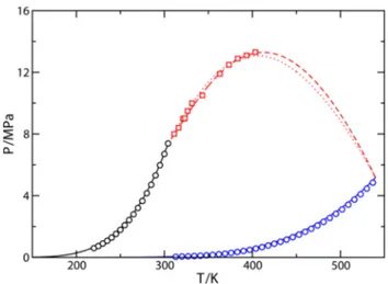
RESULTS AND DISCUSSIONTHF + CO2Binary Mixture. The THF(1) + CO2(2) binary mixture exhibits type I phase behavior according to the van Konynenburg and Scott classification.20,21In a PT projection of the phase diagram, as shown inFigure 1, the gas−liquid critical line is continuous, running from the critical point of component 1, THF, to the critical point of component 2, CO2. In particular, there is no liquid−liquid separation in the system, or in other words, the liquid mixture of THF and CO2 is homogeneous at any composition. We first determine the critical line of the mixture from the molecular parameters of the pure components in order to assess the ability of SAFT VR, in conjunction with the Berthelot rule given byeq 4for the unlike dispersive interactions with ξ12 = 1, in predicting the critical behavior of the system.
It is important to recall here that we are using rescaled molecular parameters to the critical points of pure components to obtain the best possible representation of the critical behavior of the system. However, this produces an accuracy loss in the calculated saturated liquid density of pure components, as it has been shown in previous works.29,30,36,70 However, these sets of parameters provide a good description of the coexistence compositions and critical curves. A more satisfactory description of these systems could be obtained using the versions of SAFT VR proposed by McCabe and Kiselev, using a crossover treatment,71,72 or the more recent versions of Forte et al.,73,74 in combination with the renormalization group theory.
As can be seen inFigure 1, agreement between experimental data taken from the literature and predictions from the theory is good in the whole range of compositions, especially taking into account that SAFT VR results are pure predictions. However, it seems that the shape of the continuous gas−liquid critical line is not captured by the theoretical predictions, especially near the maximum of the critical curve. Unfortunately, no experimental data for temperatures above 400 K are available. In order to obtain more accurate results, we have adjustedξ12to improve the description of the gas−liquid critical line of the mixture. The value obtained (ξ12 = 0.95) is treated as temperature independent and used to study the complete pressure− temperature−composition (PTx) phase behavior of the mixture in a wide range of thermodynamic conditions. As can be seen, agreement between theoretical results and experimental data taken from the literature for the gas−liquid critical line is excellent in the whole range of temperatures with available experimental data.
Figure 2 shows the Px slices of the phase diagram at temperatures varying from 298 to 353 K, approximately, compared with experimental data taken from literature. We have determined the phase behavior of the mixture using two different values of the binary unlike dispersive energy parameter,ξ12= 1, which corresponds to the original Berthelot value for the dispersive energyϵ12, andξ12= 0.95, a value found to give the optimal representation of the gas−liquid critical line. As can be seen, the mixture is subcritical at the lowest temperature considered, 298.15 K, since it is below the critical temperature of CO2 (Tc≈ 304 K). Both values of ξ12 give a good representation of the Px slices at different temperatures, although calculations obtained using ξ12 = 0.95 are clearly better than those predicted usingξ12= 1. In particular, SAFT VR estimations provide similar values of composition along the gas branch of the phase envelope at nearly all temperatures considered. Notice, however, that theoretical results slightly overestimate the composition of THF in the gas phase at 353 K, especially at low pressures (p ≈ 2 MPa). Predictions
Figure 1. PT projection of the phase diagram for the THF(1) + CO2(2) binary mixture. The blue and black circles correspond to the experimental vapor pressure data of pure THF61and pure CO2,62−67 respectively, and red squares68,69 to the experimental gas−liquid critical line. The continuous black and blue curves are the SAFT VR calculations for the vapor pressures, and the dotted and dashed red curves are the predictions from SAFT VR, in conjunction with the Berthelot rule, for the critical line using ξ12 = 1 and ξ12 = 0.95, respectively.
corresponding to the liquid branch of the phase diagram are clearly different when using different values of the unlike dispersive energy parameterξ12. This is an expected result since properties of liquids and, particularly, liquid composition along the vapor−liquid phase envelope depend critically on the unlike binary dispersive energyϵ12.
THF + CH4 Binary Mixture. In this section, we study the phase behavior of the THF(1) + CH4(2) binary mixture. As previously mentioned, the phase diagram of this system has not been investigated from the experimental point of view and no experimental data are available. We determine the phase behavior of the mixture from the SAFT VR approach using the molecular parameters of THF and CH4, and the Berthelot combining rules to evaluate the unlike dispersive energy of the system (eq 4), that is, usingξ12= 1. We follow this approach because experimental data are not available to judge the magnitude of the required correction inξ12. In addition to that, we have also obtained the phase diagram of the mixture using ξ12= 0.95. One would expect that the true value forξ12for this mixture should lie between the unity and that of the THF(1) + CO2(2) mixture, probably lying close to the latter. Hence, it would be very helpful in this regard to indicate what would happen to the phase diagram if one would chooseξ12= 0.95.
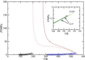
As mentioned before, the THF(1) + CH4(2) binary mixture exhibits type III phase behavior. Figure 3 shows the PT projection of the phase diagram. As can be seen, the behavior of the system is governed by a huge LL immiscibility region located at temperatures below one of the branches of thefluid− fluid critical line of the mixture and high pressures. This branch of thefluid−fluid critical line, that runs from the critical point of the heaviest component (THF), changes continuously its character from vapor−liquid (at low pressures and temper atures close to the critical point of THF) to liquid−liquid as the temperature decreases. The other branch of the gas−liquid critical line, which is very short, starts at the critical point of the
lightest component (CH4), ending at an upper critical end point (UCEP) and meeting a three phase liquid−liquid−vapor (LLV) line coming from low temperatures and pressures (see the inset ofFigure 3).
As it is well known79that the PT projection of the phase diagram corresponding to the three phase line can be located at different relative positions with respect to the vapor pressure curve of the more volatile component. In this particular case, the LLV three phase line lies entirely between the vapor pressure curves of both pure components, producing the presence of hereto azeotropy and terminating at a UCEP located at a higher temperature than the critical temperature of the lightest component. The sensitivity of the SAFT VR predictions using two different unlike dispersive interaction parameters ξ12 can be also observed in this figure. As can be seen, a decrease of the value ofξ12 (from 1 to 0.95) produces an enlargement of the liquid−liquid immiscibility region of the phase diagram, that is, for ξ12 = 1.0 THF and CH4 become immiscible at P≳ 50 MPa and P ≲ 200 K; however, for ξ12 = 0.95, the mixture exhibits liquid−liquid immiscibility below 280 K, approximately, for similar values of the pressure. This is an expected behavior since a decrease in the value ofξ12provokes unfavorable dispersive interactions between THF and CH4and, hence, a promotion of the liquid−liquid phase separation at higher temperatures.
The different VL and LL coexistence regions of the phase diagram of the THF(1) + CH4(2) binary mixture become more apparent in constant temperature Px and constant temperature Tx slices of the PTx surface. We first consider constant temperature Px slices at high temperatures and above the critical temperature of pure CH4and the UCEP of the mixture, ∼192 K.Figure 4a shows six Px slices at different temperatures. Thefive highest temperatures, that is, T ≥ 300 K, correspond to coexistence phases with gas−liquid character. As can be seen, as the temperature decreases, the gas−liquid character of the phase envelope continuously changes to a typical LL coexistence, especially at high pressures. This effect is clearly
Figure 2.Px slices of the phase diagram for the THF(1) + CO2(2) binary mixture at (a) 298.15, (b) 311, (c) 316, (d) 321, (e) 331, and (f) 353 K. The dashed and continuous curves represent SAFT VR estimations usingξ12= 1 andξ12= 0.95, respectively, and the symbols represent the experimental data taken from literature.68,75−77
Figure 3. PT projection of the phase diagram for the THF(1) + CH4(2) binary mixture. The circles correspond to the experimental vapor pressure data of pure THF61and pure CH4.78The continuous blue curves are the SAFT VR predictions for vapor pressures, the dotted and dashed red curves are the theoretical predictions for the critical lines usingξ12= 1 and 0.95, respectively, and the dashed and dotted green curves are the LLV three phase lines predicted usingξ12 = 1 and 0.95, respectively. The inset shows the region close to the critical point of pure CH4.
seen as the temperature is further decreased. T = 260 K can be viewed as an intermediate temperature at which the continuous transition from VL to LL character takes place. It is important, however, to recall that this transition is not only observed at constant pressure, but also at a given temperature, and varying the pressure. This is particularly clear in the Px slice, at which the system behaves as a liquid in coexistence with its vapor at low temperature, but exhibits LL immiscibility at high pressures.
We now turn our attention to the phase behavior at much lower temperatures, close to but below the UCEP of the mixture and the critical point of pure CH4. In Figure 4b, a constant temperature Px slice at 170 K is shown. As can be seen, since temperature is below the UCEP of the system, both VL and LL phase separation are seen in the same Px slice. At low pressures, below ∼2.427 MPa, the system exhibits VL equilibria, the three phase coexistence is observed at P≈ 2.427 MPa, and a huge LL immiscibility region is seen at higher pressures. There exists a second tiny VL region above the three phase coexistence region, at THF compositions x1∼ 0.005, as can be seen in the inset of thefigure.
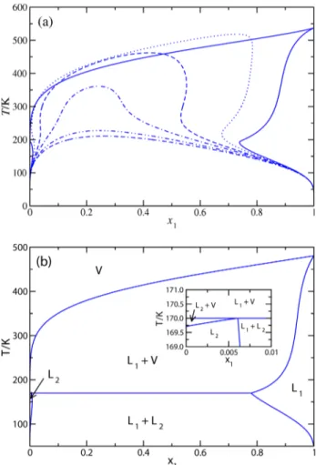
We have also studied a number of constant pressure Tx slices of the PTx phase diagram of the mixture.Figure 5a shows the
phase envelopes at different pressures, from 5 up to 75 MPa. Note that all pressures lie above the critical pressure of both components (critical pressures of pure THF and CH4are 5.02 and 4.6 MPa, respectively). The lowest pressure, 5 MPa, lies slightly below the critical pressure of pure THF. This results in a coexistence with vapor−liquid character at high temperatures and a region of liquid−liquid character at low temperatures, characteristic of mixtures that exhibit type III phase behavior. At higher pressures (from 10 up to 75 MPa), the distinction between the gas and liquid phases becomes more difficult because the two phases in coexistence are fluids (liquid like) with different densities.
We have analyzed, as in the case of the Px slices of the diagram for the binary mixture, the phase behavior at a lower pressure, 2.427 MPa, close to the UCEP of the mixture and the critical point of pure CH4. Note that this pressure corresponds to the pressure of the LLV three phase point of the system at 170 K, as discussed previously in the context ofFigure 4b. This means that the corresponding constant temperature Tx slice of the phase diagram must show a LLV three phase line at the same temperature, 170 K. As can be seen inFigure 5b, above this temperature, the system exhibits vapor−liquid phase separation, whereas below 170 K, the system separates into two immiscible liquid phases, a L1liquid phase rich in THF and
Figure 4.Px slices of the phase diagram for the THF(1) + CH4(2) binary mixture as obtained from the SAFT VR approach at (a) temperatures, from top to bottom of the relative maxima of the curves, 260, 300, 350, 400, 450, and 500 K, and (b) at 170 K. In all cases, only the Lorentz−Berthelot combining rule for the unlike dispersive interaction is used (ξ12= 1.0) . The inset of part (b) shows the region close to the three phase line in the methane rich liquid phase.
Figure 5.Tx slices of the phase diagram for the THF(1) + CH4(2) binary mixture, as obtained from the SAFT VR approach at (a) pressures, from top to bottom of the relative maximum of the curves, 5, 10, 20, 30, 50, and 75 MPa, and (b) at 2.427 MPa. In all cases, only the Lorentz−Berthelot combining rule for the unlike dispersive interaction is used (ξ12= 1.0) . The inset of part (b) shows the region close to the three phase line in the methane rich liquid phase.
a second L2liquid phase rich in CH4. As previously mentioned, at 170 K the system exhibits LLV phase separation, in agreement with results shown inFigure 4b. We have not shown the Px and Tx slices in the case ξ12 = 0.95 since a similar qualitative behavior is expected. Note that it is possible to have an approximate picture of them from a careful inspection and analysis of the PT projection of the phase diagram of the mixture shown inFigure 3.
THF + H2O Binary Mixture. Finally, we analyze in this section the phase behavior of the last mixture considered, the THF(1) + H2O(2) binary mixture. We focus on two different parametrizations used to the describe the global phase equilibria of the mixture. As we have discussed earlier, in the first case, referred to as set A, the intermolecular potential model parameters are obtained to ensure the best description of the maximum exhibited by the liquid−liquid critical line of the mixture. In the second case, referred to as set B, intermolecular potential model parameters are obtained to ensure the best description of the upper and lower critical end points of the mixture.
Figure 6shows the PT projection of the phase diagram for the THF(1) + H2O(2) binary mixture. It is immediately clear
that the SAFT VR approach, using the set A of intermolecular potential model parameters developed in this work, predicts type VI phase behavior, with a continuous gas−liquid critical line running between the critical point of the two pure components of the mixture, and a region of liquid−liquid immiscibility bounded below and above by a critical line which corresponds to the locus of the upper and lower critical solution temperatures (at different pressures). At low pressures, the liquid−liquid critical line ends at two critical end points linked by a LLV three phase line running from 314 to 420 K, approximately. In addition to that, the system exhibits positive azeotropy (the boiling point of the azeotrope is located at lower
temperatures than the boiling point temperatures of both pure components) . As can be seen inFigure 6, the azeotropic line of THF(1) + H2O(2) begins at 600 K approximately, being tangent to the continuous gas−liquid critical line of the system and runs toward lower temperatures and pressures. This azeotropic line is well above the vapor pressure curves of pure THF and H2O, including the low temperature and pressure regions (between the upper and lower critical end points of the mixture), corroborating the positive character of the azeotropy, as it is shown in the inset of the figure. This line is also close but slightly above the LLV three phase line of the system.
The THF(1) + H2O(2) system also exhibits a Bancroft point located at 480 K and 2.4 MPa, approximately. This feature is usually related to molecules that are dissimilar in chemical type or in shape but have similar vapor pressures. In this particular case, as can be seen in the Figure, the vapor pressure of H2O is higher than that of THF above 480 K, that is, H2O is more volatile than THF at high temperatures. On the contrary, below the Bancroft temperature, THF is more volatile than H2O (see both vapor pressure curves in the inset of the Figure) .
Undeniably, the most salient feature of the PT projection of the phase diagram of the THF(1) + H2O(2) binary mixture is the characteristic region of closed loop liquid−liquid immisci bility exhibited by the system. As can be seen, the mixture is completely miscible at low temperatures, below the left side liquid−liquid critical line running from the LCEP of the mixture up to high pressures, but also at high temperatures, above the right side liquid−liquid critical line running from the UCEP of the mixture up to high pressures. At intermediate temperatures, inside the region of the phase diagram located between the LLV three phase line and liquid−liquid critical line of the mixture, the system is immiscible. Note that the liquid− liquid immiscibility region is seen to disappear at a maximum in the pressure, usually called a hypercritical point.
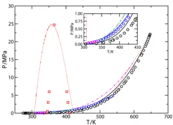
As the figure shows, the set A of intermolecular potential model parameters provides a reasonable description of the limited literature experimental data. The SAFT VR approach is able to predict the conditions at which the azeotropic line exists, in good agreement with experimental data.89Note that, as seen in the inset of thefigure, only experimental data for this line exists in the range of temperatures running form the LCEP temperature of the system up to 336 K, approximately. In addition to that, the theory is able to predict the point at which the closed loop region of liquid−liquid immiscibility for the THF(1) + H2O(2) system reaches a maximum pressure of ∼24.7 MPa, at 358 K and mixture composition x1∼ 0.214. This point, where LCST and UCST meet, is the so called hypercritical point of the mixture, as previously mentioned. This prediction is in excellent agreement with experimental values taken from literature, for which the maximum pressure, 24.7 MPa, is reached at 365 K and mixture composition x1= 0.22.23Thus, deviations between theory and experiment for the hypercritical point temperature and composition are as low as 1.4% and 2.7%, respectively.
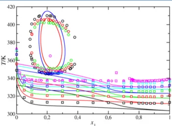
We have also compared the predictions obtained from the SAFT VR EoS with literature experimental data corresponding to the temperature−composition Tx slices of the phase diagram at conditions at which the system exhibits liquid−liquid immiscibility. As can be seen in Figure 7, the set A of intermolecular potential model parameters presented in the previous section provides a reasonable description of the experimental liquid−liquid coexistence data in a wide range of
Figure 6. PT projection of the phase diagram for the THF(1) + H2O(2) binary mixture. The curves are the SAFT VR predictions using the set A of intermolecular potential model parameters and the symbols are the literature experimental data. The black and blue circles correspond to the experimental vapor pressure data of pure THF61 and pure H2O,80−88 the red squares are the UCST and LCST at different pressures,23,24and the magenta diamonds are the azeotropic points.89 The continuous black and blue curves are the SAFT VR predictions for the vapor pressures of THF and H2O, respectively, the red dotted curves are the critical lines, the green dashed curve is the LLV three phase line, and the magenta dot dashed curve is the azeotropic line.
experimental LCEP and UCEP associated with the liquid− liquid immiscibility of the mixture. In thefirst case, in addition to an excellent description of the PT coordinates of hypercritical point of the mixture, the set A parameters are also able to predict reasonably well the width in compositions of the liquid−liquid immiscibility close loops at all the pressures considered. However, predictions of the LCST and UCST are not so accurate. In particular, SAFT VR over estimates and underestimates the LCST and UCST at all conditions, respectively. On the contrary, in the second case, in which the set B of intermolecular potential model parameters is used, agreement between theory and experiment is very good for the UCEP and LCEP of the mixture, as well as for the LCST and UCST of the system at all pressures considered; however, the predictions for the hypercritical point of the mixture and the width in compositions of the close loop diagrams are clearly in worse agreement with experiment. One may be tempted to obtain different sets of model parameters for predicting all the properties mentioned above: the hypercritical point and the UCEP and LCEP of the system, as well as the LCST and UCST and the width in compositions corresponding to the liquid−liquid immiscibility close loops. Is this ideal compromise possible? Certainly, using an analytical based EoS, such as SAFT VR or any other version that predicts classical behavior near critical regions, the answer is no.
It is important to recall here that we are using molecular parameters of pure components that have been rescaled to the experimental critical temperature and pressure. This allows using them to provide a good description of the coexistence compositions and critical curves. However, the use of these parameters produces a detriment in the calculated saturated liquid density of pure components, as it has been shown in previous works.30,70,94 In summary, one may have a set of parameters describing accurately the critical region (i.e., rescaled parameter) but with a poor description of the phase envelope at temperatures and pressure below the critical point, or a different set of parameters that predict precisely the phase envelope of the system (i.e., the usual optimized molecular parameters) but giving a poor description of the critical region.
Similarly to that, systems that exhibit liquid−liquid immisci bility close loops, as in the case of the THF(1) + H2O(2) mixture, present the same problem. The sets A and B are able to describe reasonably well the experimental data taken from the literature associated with different regions and properties, but they are not able to predict all the magnitudes of interest within the whole phase diagram of the mixture. As in the case of pure systems and binary mixtures that exhibit vapor−liquid phase behavior, a more satisfactory description of these systems could be obtained using a version of SAFT in combination with the renormalization group theory or crossover treat ment.71−74,95
We have also used the set B of molecular parameters to predict the vapor−liquid phase equilibria of the THF(1) + H2O(2) binary mixture at low pressures.Figure 10a shows the pressure−composition Px slices of the phase diagram at two different temperatures, both below the temperature lower critical end point of the mixture (TLCEP≈ 344.95 K). As can be seen, the system exhibits positive azeotropy at both temper
Figure 9.Tx closed loops regions of liquid−liquid immiscibility for the THF(1) + H2O(2) binary mixture. The symbols and curves correspond to experimental data taken from the literature23,24,47and SAFT VR estimations using set B of molecular parameters, respectively, at pressures equal to 0.1 (black circles), 0.5 (red squares and continuous red curve), 3 (green diamonds and dashed green curve), and 6 MPa (orange triangles). The magenta star corresponds to the experimental hypercritical point at 24.7 MPa.
Figure 10.(a) Px and (b) Tx slices of the phase diagram for the THF(1) + H2O(2). The symbols are the experimental data taken from the literature and curves are the predictions from SAFT VR using the set B of intermolecular potential model parameters at (a) 323.15 (blue circles22and continuous blue curve) and 343.15 K (red squares22and red dashed curve); (b) 0.04 (black circles89 and continuous black curve), 0.0533 (red squares89 and red dotted curve), 0.067 (green diamonds89 and green dashed curve), 0.08 (blue up triangles89 and blue dot dashed curve), 0.093 (magenta left triangles89 and magenta long dashed curve), and 0.1013 MPa (orange triangle down,89orange triangle right,92and orange plus,93and orange dot long dashed curve).
atures, at x1≈ 0.86 and P ≈ 0.062 MPa (T = 323.15 K) and x1 ≈ 0.78 and P ≈ 0.126 MPa (T = 343.15 K). Although SAFT VR is able to predict the existence of this behavior, the theory overestimates the pressures at which the system exhibits vapor−liquid separation. In particular, the EoS overestimates the pressure at the azeotropic point.
We have also considered the temperature−composition Tx slices of the phase diagram at low pressures, from 0.04 up to 0.1013 MPa. Unfortunately, only experimental data corre sponding to the liquid side of the phase diagram are available in literature. As can be seen inFigure 10b, predictions obtained from SAFT VR are able to predict the behavior of the mixture at low pressures. One should take into account that the set of intermolecular potential model parameters used has not been fitted to predict the vapor−liquid phase behavior but to describe accurately the lower and upper critical end points of the mixture.
Figure 11shows the temperature−composition Tx slices of the phase diagram at low and high pressures, showing the
vapor−liquid coexistence at pressures below 0.1 MPa and the closed loops of liquid−liquid immiscibility at pressure above 0.1 MPa. As can be seen, the SAFT VR approach in combination with the set B of molecular parameters is able to provide an excellent global description of the Tx slices of the phase diagram. It is important to recall again that the set B of molecular parameters have been used to provide the best possible description of the UCEP and LCEP of the mixture. However, this parametrization allows to describe reasonably well the whole phase diagram of the mixture.
Finally, we have also represented composition−composition x1y1slices of the phase diagram at 303.15 K and 0.101325 MPa.
Figure 12 shows the comparison between experimental data taken from the literature and SAFT VR predictions using the
set B of intermolecular potential model parameters. As can be seen, the theory is able to capture qualitatively the shape of the curves at the temperatures considered.
■
CONCLUSIONSA global view of thefluid phase behavior of the THF + CO2(2), + CH4(2), and + H2O(2) binary mixtures is given using the SAFT VR approach. We use a simple united atoms approx imation to model CO2and CH4molecules as chains formed by attractive spherical segments tangentially bonded and a single sphere interacting via SW potentials, respectively. The H2O molecule is modeled as spherical with four off center association sites (two sites are type H and two of type O). The THF molecule is also modeled as a chain formed by attractive spherical segments tangentially bonded together and interacting through the same type of intermolecular potential. Standard arithmetic combining rules are used to obtain the unlike segment size and potential range mixture parameters. We have also used standard geometric combining rules for the unlike energy parameter in most cases, although this parameter has also adjusted according to the modified geometric mean rule to give the best representation of the globalfluid phase behavior of some mixtures. In addition to that, two different mixture models have been developed to account for specific interactions (hydrogen bonding) between THF and H2O molecules. The first set of intermolecular potential model parameters ensures an accurate description of the maximum exhibited by the liquid−liquid critical line of the mixture at high pressures (location of the hypercritical point), whereas the second one allows the best possible description of the upper and lower critical end points of the mixture at low pressures.
We have used the mixture models to predict thefluid phase behavior of the binary mixtures containing THF. We first examine the phase diagram of the simplest system, the THF(1) + CO2(2) binary mixture, using two different mixture parameters. A set in which unlike mixture parameters are fully predicted from the molecular parameters of pure
Figure 11.Tx slices of the phase diagram for the THF(1) + H2O(2). The symbols are the experimental data taken from the literature and curves are the predictions from SAFT VR using the set B of intermolecular potential model parameters at low pressures (vapor− liquid equilibria), 0.04 (black squares89and black continuous curve), 0.0533 (red squares89 and red continuous curve), 0.067 (green squares89and green continuous curve), 0.08 (blue squares89and blue continuous curve), 0.093 (light blue squares89and light blue curve), and 0.1013 MPa (magenta up triangles,89magenta squares,92magenta diamonds,93 and magenta continuous curve), and at high pressures (liquid−liquid closed loops), 0.1 (black circles), 0.5 (blue circles and continuous blue curve), 3 (red circles and red curve), and 6 MPa (green circles). The magenta circle corresponds to the experimental hypercritical point at 24.7 MPa. Experimental data have been taken from literature.23,24,47
Figure 12.x1y1slices of the phase diagram for the THF(1) + H2O(2) binary mixture. The symbols are experimental data taken from the literature and curves are SAFT VR estimations using the set B of intermolecular potential model parameters at 0.101325 MPa (blue circles92and continuous blue curve) and 303.15 K (red squares96and
components and the original arithmetic and geometric combining rules, and a second one in which the unlike dispersive energy parameter isfitted to give the best possible representation of the continuous gas−liquid critical line of the mixture. Both theoretical results are able to describe accurately the critical line of the mixture. In addition to that, we have also examined the pressure−composition Px slices of the phase diagram at several temperatures. In all cases, agreement between theory and experiment is excellent for both sets of parameters, although the second set is able to provide a more accurate description of the mixture behavior.
We have also analyzed thefluid phase behavior of the second mixture, THF(1) + CH4(2). Unfortunately, there is no experimental data in the literature for this mixture. The theory predicts type III phase behavior for the mixture, that is, a more complex phase diagram than the previous mixture, including now a continuous liquid−liquid critical line running from the upper critical end point of the system to the critical point of pure THF, and afluid−fluid critical line that starts at the critical point of pure H2O and extends toward high pressures. The theoretical predictions indicate that the system exhibits a huge region of liquid−liquid immiscibility at low temperatures and a vapor−liquid−liquid three phase line at low temperatures and pressures, as expected for a mixture that exhibits type III phase behavior.
Finally, we have determined the high pressure phase behavior of the THF(1) + H2O(2) binary mixture using two sets of molecular parameters developed to account for the specific interactions (hydrogen bonding) between THF and H2O molecules. The theoretical results correspond to type VI phase behavior, in agreement with experimental data. In particular, the theory, using both sets of molecular parameters for association, accounts for the presence of the Bancroft point, the existence of positive azeotropy, and the closed loop liquid− liquid immiscibility of the mixture. Thefirst set of parameters, obtained to provide the best possible description of the hypercritical point of the mixture, is able to predict reasonably well the closed loop liquid−liquid immiscibility, and partic ularly, its width in compositions at different pressures. The second set, however, which has been calculated to account for accurately the upper and lower critical end points of the mixture, also predicts qualitatively the shape of the closed loops, particularly the upper and lower critical solutions temperatures of the mixture at all pressures considered. We have also studied the vapor−liquid phase equilibria at low pressures and temperatures using the set B of model parameters. All the calculations show good qualitative agree ment with experimental data.
It is important to emphasize how a simple molecular approach, such as the SAFT VR formalism, is able to account for the global phase behavior of the THF(1) + CO2(2), + CH4(2), and + H2O(2) binary mixtures, relying on very limited experimental mixture information and only one or two adjustable mixture parameter. Three of the four components considered in this work, THF, CO2, and H2O, are not particularly easy to model. In particular, THF and H2O have strong electric dipole moments and CO2 has a permanent electric quadrupolar moment. The good overall agreement we observe in the comparison with experimental data suggests that the approach used in this work contains the essential ingredients to predict the most important features of the properties studied.
As a final comment, it is interesting to mention that the results obtained in this work have been used to provide detailed information for a Molecular Dynamics study of the interfacial properties of these mixtures. In particular, the vapor−liquid and liquid−liquid coexistence data of the binary mixtures is being used as initial guesses to set up the molecular simulation boxes of interfaces involving THF + CO2, + CH4, and + H2O mixtures. This will provide important information on how united atoms realistic simulation models available in the literature may predict accurately the interfacial properties of these mixtures, with particular emphasis on interfacial tension. Note that this property is probably one of the most sensitive thermodynamic property to the molecular details of a model and it allows to check its capability for predicting other thermodynamic properties. The second stage of our long term goal, that is, the selection of appropriate molecular simulation models for determining the phase equilibria and interfacial properties of these mixtures, allows to check which of the realistic molecular models under current study will be used to simulate the phase equilibria of clathrate hydrates in a near future.
■
AUTHOR INFORMATIONCorresponding Author
*Phone: +34 959219796. Fax: +34 959219777. E mail:felipe@ uhu.es.
Notes
The authors declare no competingfinancial interest.
■
ACKNOWLEDGMENTSWe acknowledge Ministerio de Economı́a y Competitividad of Spain for financial support from Projects FIS2012 33621 and FIS2015 68910 P (M.M.P. and J.M.M.) and FIS2013 46920 C2 1 P (F.J.B. and J.A.), both cofinanced with EU Feder funds. J.M.M. acknowledges Xunta de Galicia for a Postdoctoral Grant (ED481B2014/117 0). The French CARNOT Institute ISIFoR is also acknowledged for the funds provided through the THEMYS Project (novel approaches in thermodynamical modelling and molecular simulation for the study of gas hydrates and their applications). Furtherfinancial support from Universidad de Huelva and Junta de Andalucı́a is also acknowledged.
■
REFERENCES(1) Larsen, R.; Knight, C. A.; Sloan, E. D. Clathrate Hydrate Growth and Inhibition. Fluid Phase Equilib. 1998, 150, 353−360.
(2) Sloan, E. D.; Koh, C. Clathrate Hydrates of Natural Gases, 3rd ed.; CRC Press: Boca Raton, FL, 2008.
(3) Torré, J. P.; Haillot, D.; Rigal, S.; de Souza Lima, R. W.; Dicharry, C.; Bedecarrats, J. P. 1,3 Dioxolane Versus Tetrahydrofuran as Promoters for CO2Hydrate Formation: Thermodynamics Properties, and Kinetics in Presence of Sodium Dodecyl Sulfate. Chem. Eng. Sci. 2015, 126, 688−697.
(4) Makino, T.; Sugahara, T.; Ohgaki, K. Stability Boundaries of Tetrahydrofuran + Water System. J. Chem. Eng. Data 2005, 50, 2058− 2060.
(5) Torré, J. P.; Dicharry, C.; Broseta, D. CO2Enclathration in the Presence of Water Soluble Hydrate Promoters: Hydrate Phase Equilibria and Kinetic Studies in Quiescent Conditions. Chem. Eng. Sci. 2012, 82, 1−13.
(6) Lee, Y. J.; Kawamura, T.; Yamamoto, Y.; Yoon, J. H. Equilibrium Studies of Tetrahydrofuran (THF) + CH4, THF + CO2, CH4+CO2, and THF + CO2+CH4Hydrates. J. Chem. Eng. Data 2012, 57, 3543− 3548.
(7) Florusse, L. J.; Peters, C. J.; Schoonman, J.; Hester, K. C.; Koh, C. A.; Dec, S. F.; Marsh, K. N.; Sloan, E. D. Stable Low Pressure Hydrogen Clusters Stored in a Binary Clathrate Hydrate. Science 2004, 306, 469−471.
(8) Lee, H.; Lee, J. W.; Kim, D. Y.; Park, J.; Seo, Y. T.; Zeng, H.; Moudrakovski, I. L.; Ratcliffe, C. I.; Ripmeester, J. A. Tuning Clathrate Hydrates for Hydrogen Storage. Nature 2005, 434, 743−746.
(9) Strobel, T. A.; Koh, C. A.; Sloan, E. D. Hydrogen Storage Properties of Clathrate Hydrate Materials. Fluid Phase Equilib. 2007, 261, 382−389.
(10) Struzhkin, V. V.; Militzer, B.; Mao, H. K.; Hemley, R. J. Hydrogen Storage in Molecular Clathrates. Chem. Rev. 2007, 107, 4133−4151.
(11) Veluswamy, H. P.; Kumar, R.; Linga, P. Hydrogen Storage in Clathrate Hydrates: Current State of the Art and Future Directions. Appl. Energy 2014, 122, 112−132.
(12) Kang, S. P.; Lee, H. Recovery of CO2from Flue Gas using Gas Hydrate: Thermodynamic Verification through Phase Equilibrium Measurements. Environ. Sci. Technol. 2000, 34, 4397−4400.
(13) Ricaurte, M.; Dicharry, C.; Broseta, D.; Renaud, X.; Torré, J. P. CO2 Removal from a CO2CH4 Gas Mixture by Clathrate Hydrate Formation using THF and SDS as Water Soluble Hydrate Promoters. Ind. Eng. Chem. Res. 2013, 52, 899−910.
(14) Babu, P.; Kumar, R.; Linga, P. Pre Combustion Capture of Carbon Dioxide in a Fixed Bed Reactor using the Clathrate Hydrate Process. Energy 2013, 50, 364−373.
(15) Herslund, P. J.; Thomsen, K.; Abildskov, J.; von Solms, N.; Galfre, A.; Brantuas, P.; Kwaterski, M.; Herri, J. M. Thermodynamic Promotion of Carbon Dioxide Clathrate Hydrate Formation by Tetrahydrofuran, Cyclopentane and their Mixtures. Int. J. Greenhouse Gas Control 2013, 17, 397−410.
(16) Míguez, J. M.; dos Ramos, M. C.; Piñeiro, M. M.; Blas, F. J. An Examination of the Ternary Methane + Carbon Dioxide + Water Phase Diagram using the SAFT VR Approach. J. Phys. Chem. B 2011, 115, 9604−9617.
(17) Míguez, J. M.; Garrido, J. M.; Blas, F. J.; Segura, H.; Mejía, A.; Piñeiro, M. M. Comprehensive Characterization of Interfacial Behavior for the Mixture CO2+ H2O + CH4: Comparison between Atomistic and Coarse Grained Molecular Simulation Models and Density Gradient Theory. J. Phys. Chem. C 2014, 118, 24504−24519.
(18) Herslund, P. J.; Thomsen, K.; Abildskov, J.; von Solms, N. Application of the Cubic plus Association (CPA) Equation of State to Model the Fluid Phase Behaviour of Binary Mixtures of Water and Tetrahydrofuran. Fluid Phase Equilib. 2013, 356, 209−222.
(19) Kontogeorgis, G. M.; Voutsas, E. C.; Yakoumis, I. V.; Tassios, D. P. An Equation of State for Associating Fluids. Ind. Eng. Chem. Res. 1996, 35, 4310−4318.
(20) Scott, R. L.; van Konynenburg, P. H. Static Properties of Solutions. Van der Waals and Related Models for Hydrocarbon Mixtures. Discuss. Discuss. Faraday Soc. 1970, 49, 87−97.
(21) van Konynenburg, P. H.; Scott, R. L. Critical Lines and Phase Equilibria in Binary van der Waals Mixtures. Philos. Trans. R. Soc., A 1980, 298, 495−540.
(22) Matous, J.; Novák, J. P.; S̆obr, J.; Pick, J. Phase Equilibria in System Tetrahydrofuran(1) Water(2). Collect. Czech. Chem. Commun. 1972, 37, 2653−2663.
(23) Wallbruch, A.; Schneider, G. M. Liquid + Liquid) Phase Equilibria at High Pressures Pressure Limited Closed Loop Behavior of (Xc (CH2)(4)O+(1 X)H2O) and the Effect of Dissolved Ammonium Sulfate. J. Chem. Thermodyn. 1995, 27, 377−382.
(24) Riesco, N.; Trusler, J. P. M. Novel Optical Flow Cell for Measurements of Fluid Phase Behaviour. Fluid Phase Equilib. 2005, 228, 233−238.
(25) Giner, B.; Royo, F. M.; Lafuente, C.; Galindo, A. Intermolecular Potential Parameters for Cyclic Ethers and Chloroalkanes in the SAFT VR Approach. Fluid Phase Equilib. 2007, 255, 200−206.
(26) Giner, B.; Gascón, I.; Artigas, H.; Lafuente, C.; Galindo, A. Phase Equilibrium of Binary Mixtures of Cyclic Ethers plus
Chlorobutane Isomers: Experimental Measurements and SAFT VR Modeling. J. Phys. Chem. B 2007, 111, 9588−9597.
(27) Giner, B.; Bandrés, I.; López, M. C.; Lafuente, C.; Galindo, A. Phase Equilibrium of Liquid Mixtures: Experimental and Modeled Data using Statistical Associating Fluid Theory for Potential of Variable Range Approach. J. Chem. Phys. 2007, 127, 144513.
(28) Patel, B. H.; Paricaud, P.; Galindo, A.; Maitland, G. C. Prediction of the Salting Out Effect of Strong Electrolytes on Water + Alkane Solutions. Ind. Eng. Chem. Res. 2003, 42, 3809−3823.
(29) Blas, F. J.; Galindo, A. Study of the High Pressure Phase Behaviour of CO2+ n Alkane Mixtures using the SAFT VR Approach with Transferable Parameters. Fluid Phase Equilib. 2002, 194, 501− 509.
(30) Galindo, A.; Blas, F. J. Theoretical Examination of the Global Fluid Phase Behavior and Critical Phenomena in Carbon Dioxide+ n Alkane Binary Mixtures. J. Phys. Chem. B 2002, 106, 4503−4515.
(31) Bandrés, I.; Giner, B.; López, M. C.; Artigas, H.; Lafuente, C. Isothermal (Vapour + Liquid) Equilibrium of (Cyclic Ethers + Chlorohexane) Mixtures: Experimental Results and SAFT Modelling. J. Chem. Thermodyn. 2008, 40, 1253−1260.
(32) Nonay, N.; Giner, I.; Giner, B.; Artigas, H.; Lafuente, C. Phase Equilibrium and Thermophysical Properties of Mixtures Containing a Cyclic Ether and 1 Chloropropane. Fluid Phase Equilib. 2010, 295, 130−135.
(33) Giner, I.; Montaño, D.; Haro, M.; Artigas, H.; Lafuente, C. Study of Isobaric Vapour Liquid Equilibrium of some Cyclic Ethers with 1 Chloropropane: Experimental Results and SAFT VR Model ling. Fluid Phase Equilib. 2009, 278, 62−67.
(34) Bol, W. Monte Carlo Simulations of Fluid Systems of Water Like Molecules. Mol. Phys. 1982, 45, 605−616.
(35) Nezbeda, I.; Kolafa, J.; Kalyuzhnyi, Y. V. Primitive Model of Water II. Theoretical Results for the Structure and Thermodynamic Properties. Mol. Phys. 1989, 68, 143−160.
(36) Clark, G. N. I.; Haslam, A. J.; Galindo, A.; Jackson, G. Developing Optimal Wertheim Like Models of Water for Use in Statistical Associating Fluid Theory (SAFT) and Related Approaches. Mol. Phys. 2006, 104, 3561−3581.
(37) Jackson, G.; Chapman, W. G.; Gubbins, K. E. Phase Equilibria of Associating Fluids: Spherical Molecules with Multiple Bonding Sites. Mol. Phys. 1988, 65, 1−31.
(38) Carey, F. A. Organic Chemistry; McGraw Hill: New York, 1987. (39) Fukasawa, T.; Tominaga, Y.; Wakisaka, A. J. Phys. Chem. A 2004, 108, 59−63.
(40) Ohtake, M.; Yamamoto, Y.; Kawamura, T.; Wakisaka, A.; de Souza, W. F.; de Freitas, A. M. V. Clustering Structure of Aqueous Solution of Kinetic Inhibitor of Gas Hydrates. J. Phys. Chem. B 2005, 109, 16879−16885.
(41) Takamuku, T.; Nakamizo, A.; Tabata, M.; Yoshida, K.; Yamaguchi, T.; Otomo, T. Large Angle X ray Scattering, Small Angle Neutron Scattering and NMR Relaxation Studies on Mixing States of 1,4 Dioxane Water, 1,3 Dioxane Water, and Tetrahydrofur an Water Mixtures. J. Mol. Liq. 2003, 103, 143−159.
(42) García Lisbona, M. N.; Galindo, A.; Jackson, G.; Burgess, A. N. Predicting the High Pressure Phase Equilibria of Binary Aqueous Solutions of 1 Butanol, n Butoxyethanol and n Decylpentaoxyethylene Ether (C10E5) using the SAFT HS Approach. Mol. Phys. 1998, 93, 57− 71.
(43) Clark, G. N. I.; Galindo, A.; Jackson, G.; Rogers, S.; Burgess, A. N. Modeling and Understanding Closed Loop Liquid Liquid Immis cibility in Aqueous Solutions of Poly(ethylene glycol) Using the SAFT VR Approach with Transferable Parameters. Macromolecules 2008, 41, 6582−6595.
(44) Cristino, A. F.; Rosa, S.; Morgado, P.; Galindo, A.; Filipe, E. M. J.; Palavra, A. M. F.; de Castro, C. A. N. High Temperature Vapour Liquid Equilibrium for the (Water + Alcohol) Systems and Modelling with SAFT VR: 2. Water 1 Propanol. J. Chem. Thermodyn. 2013, 60, 15−18.
(45) Cristino, A. F.; Rosa, S.; Morgado, P.; Galindo, A.; Filipe, E. M. J.; Palavra, A. M. F.; de Castro, C. A. N. High Temperature Vapour
Liquid Equilibrium for the Water Alcohol Systems and Modeling with SAFT VR: 1. Water Ethanol. Fluid Phase Equilib. 2013, 341, 48−53.
(46) dos Ramos, M. C.; Blas, F. J. Theoretical Investigation of the Phase Behaviour of Mixtures of a Novel Family of Perfluoroalkyl Polyoxyethylene Ether Diblock Surfactants in Aqueous Solutions of Carbon Dioxide. J. Supercrit. Fluids 2010, 55, 802−816.
(47) Matous, J.; Hrncir̆ík, J.; Novák, J. P.; S̆obr, J. Liquid Liquid Equilibrium in the System Water Tetrahydrofuran. Collect. Czech. Chem. Commun. 1970, 35, 1904−1905.
(48) Gil Villegas, A.; Galindo, A.; Whitehead, P. J.; Mills, S. J.; Jackson, G.; Burgess, A. N. Statistical Associating Fluid Theory for Chain Molecules with Attractive Potentials of Variable Range. J. Chem. Phys. 1997, 106, 4168−4186.
(49) Galindo, A.; Davies, L. A.; Gil Villegas, A.; Jackson, G. The Thermodynamics of Mixtures and the Corresponding Mixing Rules in the SAFT VR Approach for Potentials of Variable Range. Mol. Phys. 1998, 93, 241−252.
(50) Hansen, J. P.; McDonald, I. Theory of Simple Liquids; Academic Press: New York, 1990.
(51) Barker, J. A.; Henderson, D. J. Perturbation Theory and Equation of State for Fluids: the Square Well Potential. J. Chem. Phys. 1967, 47, 2856.
(52) Barker, J. A.; Henderson, D. J. Perturbation Theory and Equation of State for Fluids. II. A Successful Theory of Liquids. J. Chem. Phys. 1967, 47, 4714.
(53) Barker, J. A.; Henderson, D. J. What Is Liquid? Understanding the States of Matter. Rev. Mod. Phys. 1976, 48, 587−671.
(54) Boublík, T. Hard Sphere Equation of State. J. Chem. Phys. 1970, 53, 471−472.
(55) Mansoori, G. A.; Carnahan, N. F.; Starling, K. E.; Leland, T. W. Equilibrium Thermodynamic Properties of the Mixture of Hard Spheres. J. Chem. Phys. 1971, 54, 1523.
(56) Chapman, W. G.; Gubbins, K. E.; Jackson, G.; Radosz, M. New Reference Equation of State for Associating Liquids. Ind. Eng. Chem. Res. 1990, 29, 1709−1721.
(57) Wertheim, M. S. Fluids with Highly Directional Attractive Forces. I. Statistical Thermodynamics. J. Stat. Phys. 1984, 35, 19−35. (58) Wertheim, M. S. Fluids with Highly Directional Attractive Forces. II. Thermodynamic Perturbation Theory and Integral Equations. J. Stat. Phys. 1984, 35−47, 35.
(59) Wertheim, M. S. Fluids with Highly Directional Attractive Forces. III. Multiple Attraction Sites. J. Stat. Phys. 1986, 42, 459−476. (60) Wertheim, M. S. Fluids with Highly Directional Attractive Forces. IV. Equilibrium Polymerization. J. Stat. Phys. 1986, 42, 477− 492.
(61) Safarov, J.; Geppert Rybczyńska, M.; Hassel, E.; Heintz, A. Vapor Pressures and Activity Coefficients of Binary Mixtures of 1 Ethyl 3 Methylimidazolium bis(Trifluoromethylsulfonyl)Imide with Acetonitrile and Tetrahydrofuran. J. Chem. Thermodyn. 2012, 47, 56−61.
(62) Jenkin, C. F.; Pye, D. R. The Thermal Properties of Carbonic Acid at Low Temperatures. Philos. Trans. R. Soc., A 1914, 213, 67.
(63) Sengers, J. M.; Levelt, H.; Chen, W. T. Vapor Pressure, Critical Isochore and Some Metastable States of Carbon Dioxide. J. Chem. Phys. 1972, 56, 595−608.
(64) Meyers, C. H.; van Dusen, M. S. The Vapor Pressure of Liquid and Solid Carbon Dioxide. Bur. Stand. J. Res. 1933, 10, 381−412.
(65) Webster, L. A.; Kidnay, A. J. Vapor Liquid Equilibria for the Methane Propane Carbon Dioxide Systems at 230 K and 270K. J. Chem. Eng. Data 2001, 46, 759−764.
(66) Harris, J. G.; Yung, K. H. Carbon Dioxide’s Liquid Vapor Coexistence Curve And Critical Properties as Predicted by a Simple Molecular Model. J. Phys. Chem. 1995, 99, 12021−12024.
(67) Nowak, P.; Tielkes, T.; Kleinrahm, R.; Wagner, W. Supplementary Measurements of the (P,ρ,T) Relation of Carbon Dioxide in the Homogeneous Region at T = 313 K and on the Coexistence Curve at T = 304 K. J. Chem. Thermodyn. 1997, 29, 885− 889.
(68) Im, J.; Bae, W.; Lee, J.; Kim, H. Vapor Liquid Equilibria of the Binary Carbon Dioxide Tetrahydrofuran Mixture System. J. Chem. Eng. Data 2004, 49, 35.
(69) Ziegler, J. W.; Chester, T. L.; Innis, D. P.; Page, S. H.; Dorsey, J. G. Innovations in Supercritical Fluids. ACS Symp. Ser. 1995, 608, 93− 110.
(70) Galindo, A.; Whitehead, P. J.; Jackson, G.; Burgess, A. N. Predicting the High Pressure Phase Equilibria of Water + n Alkanes Using a Simplified SAFT Theory with Transferable Intermolecular Interaction Parameters. J. Phys. Chem. 1996, 100, 6781−6792.
(71) McCabe, C.; Kiselev, S. B. A Crossover SAFT VR Equation of State for Pure Fluids: Preliminary Results for Light Hydrocarbons. Fluid Phase Equilib. 2004, 219, 3−9.
(72) McCabe, C.; Kiselev, S. B. Application of Crossover Theory to the SAFT VR Equation of State: SAFT VR for Pure Fluids. Ind. Eng. Chem. Res. 2004, 43, 2839−2851.
(73) Forte, E.; Llovell, F.; Vega, L. F.; Trusler, J. P. M.; Galindo, A. Application of a Renormalization Group Treatment to the Statistical Associating Fluid Theory for Potentials of Variable Range (SAFT VR). J. Chem. Phys. 2011, 134, 154102.
(74) Forte, E.; Llovell, F.; Trusler, J. P. M.; Galindo, A. Application of the Statistical Associating Fluid Theory for Potentials of Variable Range (SAFT VR) Coupled with Renormalisation Group (RG) Theory to Model the Phase Equilibria and Second Derivative Properties of Pure Fluids. Fluid Phase Equilib. 2013, 337, 274−287.
(75) Knez, Z.; S̆kerget, M.; Ilic, L.; Lütge, C. Vapor liquid Equilibrium of Binary CO2Organic Solvent Systems (Ethanol, Tetrahydrofuran, Ortho xylene, Meta Xylene, Para Xylene). J. Super crit. Fluids 2008, 43, 383−389.
(76) Kodama, D.; Yagihashi, T.; Hosoya, T.; Kato, M. High Pressure Vapor Liquid Equilibria for Carbon Dioxide + Tetrahydrofuran Mixtures. Fluid Phase Equilib. 2010, 297, 168−171.
(77) Li, J.; Rodrigues, M.; Paiva, A.; Matos, H. A.; de Azevedo, E. G. Vapor Liquid Equilibria and Volume Expansion of the Tetrahydrofur an/CO2 System: Application to a SAS Atomization Process. J. Supercrit. Fluids 2007, 41, 343−351.
(78) Smith, B. D.; Srivastava, R. Physical Science Data: Thermody namic Data for Pure Componentes, Part A: Hydrocarbons and Ketones; Elsevier: New York, 1986; Vol. 25.
(79) Rowlinson, J. S.; Widom, B. Molecular Theory of Capillarity; Claredon Press: Oxford, U.K., 1982.
(80) Apelblat, A. J. Volumetric Properties of Aqueous Solutions of Lithium Chloride at Temperatures from 278.15 to 338.15 K and Molalities (0.1, 0.5, and 1.0) mol kg−1. J. Chem. Thermodyn. 1999, 31, 869−893.
(81) Keyes, F. Some Final Values for the Properties of Saturated and Superheated Water. J. Mech. Eng. Sci. 1931, 53, 132−135.
(82) Abdulagatov, I. M. Measurements of the Heat Capacities at Constant Volume of H2O and (H2O + KNO3). J. Chem. Thermodyn. 1997, 29, 1387−1407.
(83) Abdulagatov, I. M. Heat Capacities at Constant Volume of Pure Water in the Temperature Range 412−693 K at Densities from 250 to 925 kg m−3. J. Chem. Eng. Data 1998, 43, 830−838.
(84) Gildseth, W. J. Precision Measurements of Densities and Thermal Dilation of Water between 5 and 80 Deg. J. Chem. Eng. Data 1972, 17, 402−409.
(85) Osborne, N. S. The Pressure of Saturated Water Vapor in the Range 100 to 374 C. Bur. Stand. J. Res. 1933, 10, 155−188.
(86) Douslin, D. R. Pressure Measurements in the 0.01−30 Torr with an Inclined Piston Gauge. J. Sci. Instrum. 1965, 42, 369−373.
(87) Egerton, A. On the Saturation Pressures of Steam (170 to 374 °C). Philos. Trans. R. Soc., A 1933, 231, 147−205.
(88) Besley, L. Vapor Pressure of Normal and Heavy Water from 273.15 to 298.15 K. J. Chem. Thermodyn. 1973, 5, 397−410.
(89) Matsuda, H.; Kamihama, N.; Kurihara, K.; Tochigi, K.; Yokoyama, K. Measurement of Isobaric Vapor Liquid Equilibria for Binary Systems Containing Tetrahydrofuran using an Automatic Apparatus. J. Chem. Eng. Jpn. 2011, 44, 131−139.