THÈSE
THÈSE
En vue de l’obtention du
DOCTORAT DE L’UNIVERSITÉ DE
TOULOUSE
Délivré par : l’Institut National Polytechnique de Toulouse (INP Toulouse) Cotutelle internationale : Université de Sherbrooke
Présentée et soutenue le 06/07/2017 par :
Majd Daroukh
Effets de la distorsion sur le bruit tonal
d’un turboréacteur moderne
Effects of distortion on modern turbofan tonal noise
CONFIDENTIEL INDUSTRIE
JURY
M. Roger Ecole Centrale Lyon Rapporteur
S. Grace Boston University Rapporteur
S. Poncet Université de Sherbrooke Rapporteur
C. Polacsek ONERA Châtillon Examinateur
J.-F. Boussuge CERFACS Examinateur
N. Gourdain ISAE Directeur
S. Moreau Université de Sherbrooke Co-directeur
C. Sensiau Safran Aircraft Engines Invité
École doctorale et spécialité :
MEGEP : Dynamique des fluides
Unité de Recherche :
Remerciements
Quel plaisir d’écrire ces quelques lignes ! Beaucoup de personnes ont contribué au bon déroulement de ces trois dernières années et le moment est venu de les remercier. Je souhaite commencer par tous les membres du jury, et en particulier les rappor-teurs Michel Roger et Sheryl Grace, pour avoir accepté d’évaluer ce travail et pour leurs remarques constructives qui ont contribué à l’améliorer.
Merci également à Safran Aircraft Engines qui a financé ce projet (remerciements particuliers à Cédric Morel et à Matthieu Fiack) et au CERFACS qui m’a ac-cueilli pendant la quasi-totalité de la thèse (merci Thierry Poinsot et Jean-François Boussuge). Je souhaite remercier tout particulièrement mes différents encadrants, Stéphane Moreau, Nicolas Gourdain, Jean-François Boussuge et Claude Sensiau, pour votre présence et votre aide tout au long de la thèse. Vous m’avez tous ap-porté quelque chose en plus d’un suivi régulier et je vous en suis très reconnaissant : merci Stéphane pour ta grande réactivité et ton aide lors de l’écriture des dif-férents papiers, merci Nicolas pour tes précieux conseils lors de la rédaction, merci Jeff pour avoir transformé mes présentations (en bien, bien sûr !) et merci Claude pour ton souci de synthèse qui m’a toujours permis de raccrocher ce que je faisais au besoin industriel. Je tiens aussi à remercier Frédéric Sicot, pour m’avoir formé aux différents outils du CERFACS en début de thèse, et Marlène Sanjosé pour (entre autres) tout le support sur Optibrui.
La majeure partie de la thèse a été faite au CERFACS où j’ai passé trois très belles années et la liste des personnes à remercier est donc très longue ! Merci à tous les séniors, et en particulier merci (beaucoup beaucoup beaucoup) à Marc Montagnac pour toute l’aide que tu m’as apportée (et pas que !). Merci à toute l’administration et en particulier à Chantal (qui a tenu sa promesse pour le mail-lot !), Michèle, Marie, Nicole et Lydia pour votre bonne humeur que vous nous transmettez tous les jours ! Merci également à toute l’équipe CSG pour le support tout au long de la thèse, avec une attention particulière à Fred et Gérard pour l’organisation de la soutenance. Un grand merci aussi à tous les thésards qui ont illuminé mes journées au CERFACS (et en dehors aussi). Merci Biolchi pour les victoires faciles à FIFA, Nico pour avoir converti mes passes clés, Dario pour tes cheveux rigolos, Mélissa aussi pour tes cheveux rigolos et Césario pour tous ces bons Japoyaki. Merci Douds pour ta contribution à l’EAC, Kelu pour tes incroyables histoires, Pedro pour le pierre-feuille-ciseaux géant et Grosnick pour avoir supporté mon attaque de tasse de café. Je pense aussi à señor Cassou, à Catchi et aux duos Franchinou & Aïchou et Luis & Francis. Je n’oublie pas les plus jeunes : Maxou, l’homme le plus gentil au monde, Tastoul le grimpeur fou, Gagarin et Quegui les éternels stagiaires, Valou le bouffeur de cajou, Fél le bouffeur de pailles et Lulu le bouffeur de tibias. Je n’oublie pas non plus les mi-jeunes mi-vieux (post-docs et jeunes séniors) : Guillaume double-pédale, Micha, Lucas, Misda, la Pech et Nico le Grenoblois. Ni ceux qui ont déjà quitté le CERFACS : Carlitos le co-bureau de folie et reporter officiel de l’EAC, Lolo la joueuse d’accordéon (incroyable !), Gaëllou, Sophie, Laure, Moff, Jarjar, Abdullah, Greg, Yannis, David, Julio, Thibault et Jéjé.
Enfin, je termine la page CERFACS par une grande pensée à tous les joueurs de mon club de coeur de toujours : l’EAC (forcément !).
J’ai également eu la chance de passer quelques mois à Sherbrooke pendant cette thèse et je voulais remercier toute l’équipe d’aéroacoustique avec qui j’ai passé de très bons moments. Merci à Marlène et à Thomas (ou Léonard ?) pour m’avoir prêté votre canapé et avoir supporté mes questions pour la DPR. Un grand merci à Vianney pour nos incroyables discussions et nos matchs de ping-pong de légende ! Merci aussi au poète Aurélien, à Dark Chaofan, Hao, Prateek, Micha, Albane et Alexis. J’ai vraiment apprécié tous les moments passés avec vous !
Je souhaite aussi remercier toute l’équipe acoustique de Safran Aircraft Engines qui m’a toujours bien accueilli à chacun de mes passages. Je pense notamment à tous ceux qui avec qui j’ai interagi pendant la thèse (Claude Sensiau, Matthieu Fiack, Cédric Morel, François Julienne, Jacky Mardjono, Anthony Laffite, Mathieu Gruber, Rasika Fernando, Johan Thisse), aux footeux (Norman Jodet et Jérémy González) et à tous les autres pour les bons moments partagés autour d’un café !
Enfin, je termine par une pensée pour mes amis parisiens que je n’ai pas beaucoup vus pendant ces trois années (big up Nono, Paul, Charles, Julien, Chami, Fabio et Farah) mais qui m’ont inspiré à chaque repas partagé. Merci à Agathe pour cette dernière année passée à mes côtés et un très grand merci à toute ma famille à qui je dois beaucoup et qui m’a toujours soutenu pendant cette thèse.
Abstract
Fuel consumption and noise reduction trigger the evolution of aircraft engines to-wards Ultra High Bypass Ratio (UHBR) architectures. Their short air inlet design and the reduction of their interstage length lead to an increased circumferential in-homogeneity of the flow close to the fan. This inin-homogeneity, called distortion, may have an impact on the tonal noise radiated from the fan module. Usually, such a noise source is supposed to be dominated by the interaction of fan-blade wakes with Outlet Guide Vanes (OGVs). At transonic tip speeds, the noise generated by the shocks and the steady loading on the blades also appears to be significant. The increased distortion may be responsible for new acoustic sources while interacting with the fan blades and the present work aims at evaluating their contribution. The effects of distortion on the other noise mechanisms are also investigated. The work is based on full-annulus simulations of the Unsteady Reynolds-Averaged Navier-Stokes (URANS) equations. A whole fan module including the inlet duct, the fan and the Inlet and Outlet Guide Vanes (IGVs/OGVs) is studied. The OGV row is typical of current engine architecture with an integrated pylon and two different air inlet ducts are compared in order to isolate the effects of inlet distortion. The first one is axisymmetric and does not produce any distortion while the other one is asym-metric and produces a level of distortion typical of the ones expected in UHBR engines. A description and a quantification of the distortion that is caused by both the potential effect of the OGVs and the inlet asymmetry are proposed. The effects of the distortion on aerodynamics are highlighted with significant modifications of the fan-blade wakes, the shocks and the unsteady loading on the blades and on the vanes. Both direct and hybrid acoustic predictions are provided and highlight the contribution of the fan-blade sources to the upstream noise. The downstream noise is still dominated by the OGV sources but it is shown to be significantly impacted by the inlet distortion via the modification of the impinging wakes.
Résumé
Les objectifs en termes de réduction de la consommation et du bruit émis par les moteurs d’avions ont progressivement mené aux architectures à très grand taux de dilution (UHBR). Leur géométrie est caractérisée par une entrée d’air courte et par une réduction de l’espace entre la soufflante et les aubes du redresseur du flux sec-ondaire (OGVs), entraînant alors une augmentation de l’inhomogénéité azimutale de l’écoulement au niveau de la soufflante. Cette inhomogénéité, appelée distorsion, pourrait impacter le bruit tonal généré par le module de la soufflante. Ce bruit est généralement supposé être dominé par le mécanisme d’interaction des sillages des pales de la soufflante avec les OGVs. En régime transsonique, le bruit de choc et le bruit de charge stationnaire deviennent également prépondérants. L’augmentation de la distorsion pourrait être à l’origine de nouvelles sources de bruit en interagissant avec les pales de la soufflante et l’objectif de cette thèse est d’évaluer leur contri-bution. Les effets de la distorsion sur les mécanismes de bruit déjà existants sont également analysés. Cette étude est réalisée à l’aide de simulations numériques des équations instationnaires de Navier-Stokes moyennées (URANS). Un module com-plet de fan est considéré sur 360 degrés et se compose d’un conduit d’entrée d’air, de la soufflante et des redresseurs des flux primaire et secondaire (IGVs/OGVs). Le redresseur du flux secondaire est typique des moteurs actuels avec un pylône inté-gré et deux entrées d’air différentes sont étudiées de manière à isoler les effets de la distorsion d’entrée d’air. La première est axisymétrique et ne produit donc pas de distorsion alors que la deuxième ne l’est pas et produit un niveau de distorsion typique de ceux attendus dans les moteurs UHBR. Une description et une quantifi-cation de la distorsion due à l’effet potentiel des OGVs et de celle due à l’asymétrie de l’entrée d’air sont proposées. Les effets de la distorsion sur l’aérodynamique sont mis en évidence avec notamment une modification importante des sillages des pales de la soufflante, des chocs et de la charge instationnaire exercée sur les différentes pales et aubes. Des prévisions acoustiques basées sur les approches directe et hy-bride sont réalisées et soulignent la contribution importante des sources localisées sur les pales de la soufflante sur le bruit amont. Le bruit aval reste dominé par les sources sur les OGVs mais est tout de même impacté par la distorsion d’entrée d’air via la modification des sillages.
Contents
Introduction 15
General context . . . 15
Noise from an aircraft engine . . . 16
Noise from a fan module . . . 18
A new source breakdown caused by distortion? . . . 22
Organization of the manuscript . . . 24
1 Methods for the prediction of fan tonal noise 27 1.1 Introduction . . . 27
1.2 Fundamentals of aeroacoustics . . . 28
1.2.1 Equations in fluid dynamics . . . 28
1.2.2 Lighthill’s analogy . . . 29
1.2.3 Linearized theory . . . 31
1.2.4 Chu & Kovasznay’s analysis . . . 32
1.2.5 Application to the prediction of fan tonal noise . . . 35
1.3 Acoustic energy . . . 38
1.3.1 Acoustic energy in a stagnant uniform fluid . . . 38
1.3.2 Acoustic energy in a homentropic non-uniform fluid . . . 41
1.3.3 Notion of acoustic power . . . 42
1.4 Direct noise predictions . . . 45
1.4.1 CFD simulations . . . 45
1.4.2 Filtering of non-acoustic perturbations . . . 47
1.5 Hybrid noise predictions: source determination . . . 48
1.5.1 Amiet’s model . . . 48
1.5.2 Extensions . . . 52
1.6 Hybrid noise predictions: sound propagation . . . 53
1.6.1 Goldstein’s analogy . . . 53
1.6.2 Extension to a slowly varying duct . . . 58
1.6.3 First-order approximation of swirl effects . . . 61
1.6.4 Further extensions . . . 62
2 Numerical simulations of a fan stage with bifurcations and inlet distortion 65 2.1 Introduction . . . 65 2.2 Engine model . . . 65 2.2.1 Geometry . . . 66 2.2.2 Operating points . . . 67
2.3 Numerical setup and convergence . . . 68
2.3.1 Numerical setup . . . 69
2.3.2 Convergence . . . 71
2.4 Basic flow features . . . 75
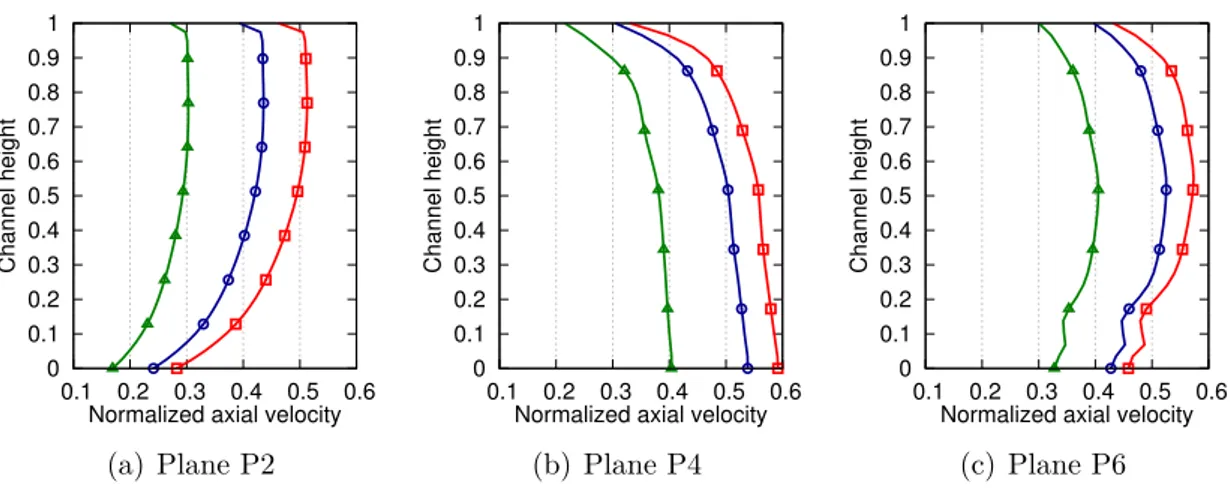
2.4.1 Extractions planes and normalization . . . 75
2.4.2 Instantaneous flow . . . 76
2.4.3 Mean flow . . . 80
2.5 Conclusion . . . 84
3 Characterization of the distortion and impact on aerodynamics 85 3.1 Introduction . . . 85
3.2 Distortion caused by the potential effect of the pylon . . . 86
3.2.1 Characterization of the potential effect near the pylon . . . 86
3.2.2 Evolution of the shape with distance . . . 88
3.2.3 Deviation with distance . . . 90
3.2.4 Decrease of the intensity with distance . . . 92
3.2.5 Radial evolution . . . 93
3.2.6 Distortion downstream of the stators . . . 95
3.3 Distortion caused by the inlet asymmetry . . . 96
3.3.1 Characterization of the inlet distortion . . . 96
3.3.2 Evolution of the shape with distance . . . 99
3.3.3 Evolution of the intensity with distance . . . 101
3.3.4 Radial evolution . . . 102
3.4 Impact of distortion on unsteady aerodynamics . . . 104
3.4.1 Fan-blade wakes . . . 104
3.4.2 Blade and vane unsteady loadings . . . 108
3.4.3 Fan-blade shocks . . . 116
3.5 Conclusion . . . 118
4 Impact of distortion on acoustics 119 4.1 Introduction . . . 120
4.2 Interaction of fan-blade wakes with OGVs . . . 120
4.2.1 Analysis of the unsteady loadings . . . 120
4.2.2 Propagation in an annular duct . . . 122
4.2.3 Effect of stator heterogeneity . . . 123
4.2.4 Influence of the regime . . . 124
4.2.5 Effect of axial variation of flow and duct . . . 125
4.2.6 Effect of swirling flow . . . 127
4.2.7 Noise penalty induced by inlet distortion . . . 128
4.3 Interaction of distortion with fan blades . . . 131
4.3.2 Propagation in an annular duct . . . 132
4.3.3 Assessment of the rotor homogeneity . . . 133
4.3.4 Influence of the regime . . . 135
4.3.5 Effect of axial variation of flow and duct . . . 136
4.3.6 Power formulation . . . 137
4.3.7 Effect of swirling flow . . . 138
4.3.8 Noise penalty induced by inlet distortion . . . 139
4.4 Interaction of fan-blade wakes with IGVs . . . 142
4.4.1 Propagation in duct and assessment of the stator homogeneity 142 4.4.2 Noise penalty induced by inlet distortion . . . 143
4.5 Source breakdown using hybrid methods . . . 145
4.5.1 Source breakdown at approach . . . 145
4.5.2 Source breakdown at cutback . . . 146
4.5.3 Source breakdown at sideline . . . 148
4.6 Direct acoustic analysis . . . 150
4.6.1 Direct evaluation of acoustic power . . . 150
4.6.2 Analysis of upstream power . . . 152
4.6.3 Filtering of hydrodynamic fluctuations . . . 159
4.6.4 Analysis of downstream power . . . 169
4.7 Conclusion . . . 173
Conclusions and perspectives 175 Recalling the objectives . . . 175
Conclusions from a physical point of view . . . 175
Conclusions from a methodological point of view . . . 177
Future work . . . 178
A Add-ons for the numerical simulations 187 A.1 URANS formalism . . . 187
A.2 Turbulence modeling . . . 189
A.3 Discretization of the equations . . . 191
B Add-ons for Goldstein’s analogy 197 B.1 Derivation of the duct modes . . . 197
B.2 Derivation of the duct Green’s function . . . 200
B.3 Simplification of the source term . . . 202
C One-dimensional validation of the numerical setup 207 C.1 Propagation of acoustic waves . . . 207
C.2 Stretching zones . . . 208
D Effects of mesh refinement 211 D.1 Effects on aerodynamic patterns . . . 211
D.2 Effects on noise predictions . . . 213
List of symbols
Latin characters
a0 Speed of sound of the uniform flow
Amn Weight of Jm(αmnr)
b Half-chord
B Number of rotor blades
Bmn Weight of Ym(αmnr)
D Acoustic energy dissipation or fan diameter depending on the context
E Acoustic energy density
fi Components of pressure force vector
g Amiet’s transfer function
G Green’s function
h Position height
H Total vane height
Ix Acoustic energy flux along the x-axis
I Acoustic energy flux
Jm Bessel function of the first kind of order m
k0 Wavenumber of the uniform flow
kmn Defined by kmn2 = k20− β02α2mn
kx Spatial wavenumber along the x-direction
ky Spatial wavenumber along the y-direction
L Distance to the fan L
m Azimuthal order
M0 Axial Mach number of the uniform flow
n Radial order
n Normal vector to the wall
pmn Pressure of the mode (m, n)
Ps Acoustic power carried by the sth harmonic
Rh Hub radius
Rt Tip radius
S Source surface
Smn Source term of the mode (m, n)
t Receiving time
umn Axial velocity of the mode (m, n)
U0 Axial velocity of the uniform flow
V Number of stator vanes
w Upwash
X Slowly varying observer axial coordinate x Observer position, also written (xi) or (x, r, θ)
Y Slowly varying source axial coordinate
Ym Bessel function of the second kind of order m y Source position, also written (yi) or (y, ry, θy)
Greek characters
αmn Radial eigenvalue of the mode (m, n)
β0 Defined by β02 = 1 − M02
γmn Axial wavenumber related to the mode (m, n) Γmn Norm of the duct eigenfunction Ψmn
δ Dirac’s distribution
∆P Pressure jump over the airfoil
ρ0 Mean density
ρmn Density of the mode (m, n)
τ Emission time
Ψmn Duct eigenfunction of the mode (m, n)
ω Pulsation
Ω Engine rotational speed
Indices and superscripts
m Azimuthal mode order
n Radial mode order
s Harmonic order
0 Mean flow values
′ Fluctuating values
+ Upstream value
− Downstream value
Acronyms
BPF Blade Passing Frequency
BPR ByPass Ratio
CAA Computational AeroAcoustics
CDC Circumferential Distortion Coefficient CFD Computational Fluid Dynamics DNS Direct Numerical Simulation DRI Distortion-Rotor Interaction
DTS Dual Time Step
IGV Inlet Guide Vane
LEE Linearized Euler Equations LES Large Eddy Simulations OGV Outlet Guide Vane
RANS Reynolds-Averaged Navier-Stokes RF Rotational Frequency
UHBR Ultra High Bypass Ratio
URANS Unsteady Reynolds-Averaged Navier-Stokes WSI Wakes-Stator Interaction
Introduction
General context
The environmental impacts from aviation are multiple and could lead to a critical constraint on capacity growth. Aircraft engine emissions contribute to the air qual-ity and the climate change [1] and aircraft engine noise causes health hazards to the exposed population, especially with the expansion of urban areas around airports. Standards are therefore defined by the International Civil Aviation Organization (ICAO) in support of an environmentally responsible civil aviation sector [2].
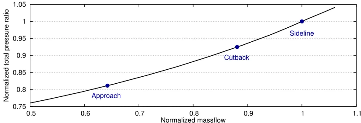
In its strand dedicated to aircraft noise, the ICAO has defined the maximum noise levels acceptable for civil aircrafts. These levels are expressed in EPNdB, a unit representative of the nuisance to airport communities. They are established from three certification points, illustrated in Fig. 1:
• one lateral point measured 450 m from the runaway at full power (sideline); • one point at 6.5 km on the extended centre line of the runaway after the
reduction of thrust (cutback);
• and one point at 2 km on the extended centre line of the runaway at low speed (approach). Approach Sideline Cutback 2000 m 450 m 6500 m 3° Maximum thrust Cutback thrust 300 m
The standards imposed by the ICAO become more restrictive to mitigate the constantly increasing air traffic. They are driven by the chapter evolution of the volume I of the ICAO report. Current standards are described in chapter 4 but the ones of chapter 14, which impose a reduction of 7 EPNdB, are being applied or will be applied by 2020 depending on the type of aircraft [2].
In addition to these certifications, Europe, via the Advisory Council for Aero-nautics Research in Europe (ACARE) has established in 2001 even more challenging goals. Thus, the subjective perception of the noise radiated by an aircraft should be reduced by 50 % in 2020 and by 65 % in 2050, relative to year 2000 average levels. This corresponds to a reduction of 30 EPNdB (10 EPNdB per certification point) and 39 EPNdB (13 EPNdB per certification point) respectively [4].
Two main contributions are identified at the three certification points: the engine noise and the airframe noise. First experimental studies have shown a domination of engine noise at high speed (cutback and sideline points), when the landing gear and the high-lift devices are not (entirely) deployed. At low speed (approach point), both the landing gear and the high-lift devices are released and are responsible for an important noise thus making the airframe and the engine noise comparable [5]. A better understanding of both sources becomes a necessity to respect the future more stringent standards. The present study focuses on the noise radiated from the engine.
Noise from an aircraft engine
The noise from an aircraft engine naturally depends on the architecture of the engine. The study is limited to turbofan engines which propel most commercial aircrafts be-cause of their high efficiency. Counter Rotating Open Rotors (CRORs) are expected to present higher propulsive efficiency but technical challenges in terms of installa-tion, noise and certification remain [6].
In a turbofan engine, the thrust is not only resulting from the burnt gases. As illustrated in Fig. 2, air is ingested (and compressed) by the fan and is split into two streams. The air of the primary stream follows the Brayton thermodynamic cycle. It is straightened by the Inlet Guide Vanes (IGV), compressed through the stages of the compressor, mixed with the fuel, burnt in the combustion chamber, expanded through the stages of the turbine and accelerated in the nozzle. The energy collected by the turbine is used to rotate the fan and the compressor. As for the air of the secondary stream, it is directly straightened by the Outlet Guide Vanes (OGV) and accelerated through the nozzle.
Both streams contribute to provide thrust: the primary stream by accelerating the flow and the secondary stream by ingesting an air mass-flow rate. The ratio between the mass-flow rate of air in the secondary stream and the one in the pri-mary stream is called the ByPass Ratio (BPR). The higher the BPR, the lower the fuel consumption is (for a given thrust). However, the higher the BPR, the larger
Fan IGV OGV
Nacelle
Pylon
Compressor Combustor Turbine
Secondary flux
Primary flux
Figure 2: Turbofan engine architecture (reproduced from [7])
the engine is, and consequently, the higher the weight and drag are. A trade-off between engine efficiency and engine size must be done. Current classical engines are characterized by a BPR of about 5-7. The newer ones, such as the LEAP which propels the A320neo, are characterized by a BPR of about 10. They are referred to as High Bypass Ratio (HBR) engines. An optimization of this trade-off will be achieved in future engines by reducing the length of their nacelle by:
• shortening the air inlet duct;
• including the structural pylon into the OGV row; • and moving closer to the fan the OGV and the pylon.
These evolutions are schematically represented in Fig. 3. These new engines will have a BPR around 15 and are called Ultra High Bypass Ratio (UHBR) engines. They are likely the last evolution of turbofan engines before a technological break-through.
Almost all the components of a turbofan engine create some noise. Studies that have been conducted so far allows identifying three main sources of engine noise:
• the fan, compressor and turbine noise, due to the rotation of physical elements; • the jet noise, caused by the turbulent shear layer between the jet and the
ambiant air;
• and the combustion noise, essentially due to flame unsteadiness in the com-bustor and acceleration of entropy spots.
Jet noise has been the dominant source of an engine for a long time but the evolution towards higher BPR is modifying the breakdown. This is shown in Fig. 4 which shows the contribution of the main sources at the three certification points for typical HBR and UHBR engines. When increasing the BPR, the exhaust velocities become lower and the importance of jet noise starts to decrease compared to fan noise. This trend is further accentuated by the short nacelle design in UHBR engines whichs reduces the surface available for acoustic treatments [6].
Fan Nacelle
(a) Increase of nacelle diameter Fan Nacelle (b) Shortening of air inlet duct Fan Nacelle OGV Pylon
(c) Reduction of space between the fan and the OGV Figure 3: Evolution towards UHBR architectures
Noise from a fan module
The study focuses on the noise radiated by the fan which becomes the main issue (in terms of acoustics) in UHBR engines because of its contribution at all certifi-cation points. Typical noise spectra of a fan operating at subsonic and supersonic conditions are given in Fig. 5. At both operating conditions, the noise is com-posed of a tonal contribution and a broadband one. At subsonic tip speeds, the broadband noise generated by the fan is expected to be larger than the tonal noise. Tones emerge at the Blade Passing Frequency (BPF) fBP F = BΩ/2π, where B is the number of fan blades and Ω is the shaft-rotational speed. Their levels are above the broadband noise level by a few tens of decibels. At supersonic tip speeds, the trend is generally reversed and the tonal noise dominates. A lot of additional tones, called Multiple Pure Tones (MPT) and linked to the Rotational Frequency (RF)
fRF = Ω/2π, become significant.
Sources of fan tonal noise
The main mechanisms that are responsible for tonal noise are schematically repre-sented in Fig. 6 and can be classified into three categories that are detailed below [6].
Jet 5 % Fan 35 % Airframe 60 % Jet 20 % Fan 65 % Airframe 15 % Jet 30 % Fan 70 %
Approach Cutback Sideline
BPR ∼10 (a) HBR engine Combustion 5 % Fan 50 % Airframe 45 % Combustion 15 % Jet 10 % Fan 75 % Combustion 5 % Jet 20 % Fan 75 %
Approach Cutback Sideline
BPR ∼15
(b) UHBR engine
Figure 4: Source breakdown at certification points for typical HBR and
UHBR engines (Safran estimates)
Frequency (Hz)
Noise level (dB)
10 dB
BPF harmonics
Broadband spectrum
(a) Subsonic fan
Frequency (Hz) Noise level (dB) 10 dB BPF harmonics Broadband spectrum MPT (b) Supersonic fan
Figure 5: Typical noise spectrum from a subsonic fan and a supersonic fan
(reproduced from [7])
Rotor self-noise
Rotor self-noise is the noise generated by the rotor itself, without interacting with its environment. One part of this noise is produced by the force and volume-displacement effects exerted by the rotating blades on the fluid. It is linked to the steady loading on fan blades which propagates because of the rotational motion.
Shock waves
Fan-blade wakes-OGV/IGV interaction Inlet distortion-fan interaction
Fan-blade steady loadings
Pylon/OGV/IGV potential effect-fan interaction
Figure 6: Mechanisms generating fan tonal noise (reproduced from [7])
A fan with B identical blades will produce noise at harmonics of the BPF. The resulting sound field can be decomposed into azimuthal Fourier harmonics of order equal to multiples of B (more details in Sec. 1.6.1). These modes cannot propagate through the duct at subsonic fan-tip speeds but are dominant as soon as the latter becomes supersonic (at takeoff conditions typically) [8].
In addition to this mechanism, shocks also start to develop at these supersonic tip speeds. These shocks rotate with the fan and should have the periodicity of the number of blades B. In reality, small blade-to-blade geometry variations exist because of the manufacturing and the assembly of the blades and are responsible for significant variations in shock strength. Therefore, the shocks combine together while propagating thus causing the loss of original periodicity. This results in a noise at harmonics of the RF which is often referred to as Buzz-Saw Noise (BSN). These shocks propagate only in the upstream direction and are generally responsible for an important increase of the total noise [9].
Rotor-stator interaction noise
Rotor-stator interaction noise is the noise caused by the impact of rotor-blade wakes on the stator vanes. The fan-blade wakes are steady in the rotor frame and lead to a rotating field with azimuthal orders that are multiples of the number of blades B in the stationary frame. They interact with the OGV located downstream and are responsible for unsteady lift variation. A noise is produced, again at BPF harmon-ics. Contrary to fan self-noise, a wide range of azimuthal orders is created. They correspond to the so-called Tyler & Sofrin modes m = nB − kV where V is the number of vanes, n the order of the BPF harmonic and k any integer [10]. This formula is valid when the stator vanes are all identical and evenly spaced. In cur-rent engines, the OGV is heterogeneous and all azimuthal orders could be generated (replacement of V by 1 in Tyler & Sofrin formula) [11]. Fan-IGV interaction noise is generally neglected but fan-OGV interaction is considered to be the main source of fan tonal noise [6].
Distortion-rotor interaction noise
Distortion-rotor interaction noise is caused by the impact of a stationnary circum-ferential inhomogeneity of the flow (called distortion) with the rotating fan. When the air inlet is not axisymmetric or when the potential effect of the downstream pylon is significant, the flow contains components of low azimuthal order, typically from m = −5 to m = 5. These components will be unsteady in the rotating frame and will interact with the fan blades, creating unsteady lift variations. A noise is produced at harmonics of the BPF if all blades are identical and the resulting sound field can be decomposed into azimuthal orders going from m = nB − 5 to
m = nB + 5. This noise mechanism is generally neglected for current engine
archi-tectures in which the inlet duct and the interstage are sufficiently long to attenuate both the inlet distortion and the potential effect of the pylon.
A noise can also be produced by the interaction of the fan with the potential effect of the stators (OGV and IGV). If the potential effect of these stators is important enough, the flow contains azimuthal harmonics of order equal to multiples of the number of vanes V . These components are unsteady in the rotor frame and are responsible for unsteady lift variations on the blades. The resulting sound field can be decomposed into azimuthal harmonics of order given by Tyler & Sofrin law
m = nB − kV where V is the number of vanes, n the order of the BPF harmonic
and k any integer. These noise mechanisms are generally neglected because they are considered much less important than rotor-stator interaction [6].
Sources of fan broadband noise
Historically, fan broadband noise has been less studied than fan tonal noise. Exper-imental studies have allowed for the identification of the main sources, which are linked to turbulent phenomena [12]. They are schematically represented in Fig. 7. Again, they can be classified into three categories detailed below.
Tip clearance noise Fan-blade wakes-OGV/IGV interaction Inlet turbulence-fan interaction
Fan self-noise
Boundary layers-fan interaction
Figure 7: Mechanisms generating fan broadband noise (reproduced from
Rotor self-noise
The fan itself produces noise even when it is isolated from its environment. This noise comes from the passage of the turbulent boundary layer over the trailing edge of each blade. The interaction between the turbulent and the trailing edge eddies amplifies the quadrupole noise associated with the fluid motion in a plane normal to the edge [13]. This source is a significant source of fan broadband noise [6].
Rotor-stator interaction noise
The interaction of fan-blade wakes with stator vanes has been shown to be the main contributor to fan tonal noise. These wakes possess a fully turbulent component and are also responsible for nonperiodic lift variations on the blades. This results in a broadband noise which clearly dominates other broadband noise sources [6].
Turbulence-rotor interaction noise
The interaction of a turbulent flow with the rotating fan is also responsible for broadband noise. The probably most important contribution to this noise is caused by the hub and shroud boundary layers which interact with the rotating flow in the fan region. Around the casing, this noise could be very important. Its prediction is difficult and numerical simulations and experiments show humps around multiples of BPF, which might indicate the presence of noise-generating structures with a range of length scales in the boundary layer [14,15].
Another source comes from the interaction of the inlet turbulence with the fan. The vortices of atmospheric turbulence are stretched out while ingested by the fan. When the scale of the vortices becomes high compared with the fan-blade chord, the interaction mechanism becomes coherent. Therefore, it can be seen as a distorsion-rotor mechanism and the resulting noise is mainly tonal. However, the small-scale vortices are responsible for non-coherent lift variations on the blades and result in a broadband noise.
Finally, the tip clearance noise can also be seen as an interaction mechanism between a turbulent flow and the fan. The mechanism is actually one of the most complex one. The tip clearance flow interacts with the casing boundary layer and generates tip leakage vortices. The latter interact with the blades and create un-steady lift variations which result in a broadband noise. The effect of tip clearance on the noise is not completely understood but it seems to alter both the fan-self noise and the casing boundary layer-fan interaction noise mechanisms [12, 16].
A new source breakdown caused by distortion?
The study focuses on fan tonal noise. In regular flow conditions and current architec-tures, it is dominated by the fan-OGV interaction (called here WSI for Wakes-Stator Interaction) and by the fan-self noise at transonic regimes [6,17]. The noise caused by distortion-fan interaction (called here DRI for Distortion-Rotor Interaction) is
generally neglected.
However, this breakdown might change in UHBR engines where the distortion is expected to increase because of the geometrical evolutions shown in Fig. 3. The most important distortion comes from the inlet which can be asymmetric for two different reasons. The first reason is that the engine intake is not perfectly aligned with the fan axis to account for the downward deflection of the flow by the wing in cruise conditions. The other one is due to ground-clearance requirements which leads to non-circular cross sections for large engines. Due to this asymmetry, a circumferential inhomogeneity of the flow is created at the entrance of the engine. This inhomogeneity is not sufficiently damped before reaching the fan because of the reduced length of the air inlet and will interact with it. In addition to this so-called "inlet" or "upstream distortion", the potential effect of the OGV and the pylon is increased because of the reduction of space between them and the fan. This potential effect, or "downstream distortion", is stationnary and also interacts with the rotating fan. For illustration purposes, typical axial velocity contours for a clean and a distorted inflow are given in Figs. 8(a) and 8(b) respectively.
(a) Clean inflow
Axial velocity
Min Max
(b) Distorted inflow
Figure 8: Typical axial velocity contours for a clean and a distorted inflow The impact of distortion on fan noise started to be studied experimentally in the 1970s because significant differences in noise levels were measured between static and in-flight tests [18]. These differences were attributed to the ingestion of large-scale vortices by the fan which could be seen as a stationnary distortion. The studies have led to the use of a Turbulence Control Screen (TCS) in static tests to provide a clean inflow and remove the mentionned differences [19]. Since then, the studies about the impact of distortion on the noise have been put aside. They started again very recently, precisely because of the evolution of aircraft engine architectures. The complexity of the studies is increased step by step. Holewa et al. [20] studied the impact of the bifurcations (or pylon) on the fan tonal noise by means of a quasi-3D numerical simulation of a fan and an OGV with struts and bifurcations. They found that the noise generated by the DRI mechanism was negligible compared with the one generated by the WSI mechanism. However, they highlighted the influence of
the potential effects of the bifurcations on the latter. This last point was also stud-ied by Bonneau et al. [21] and Roger & Caule [22] who explained the unexpected emergence of the first BPF harmonic by the invalidity of Tyler & Sofrin’s rule [10] in the presence of an azimuthal heterogeneity. In contrast with the study of Holewa
et al. [20], Oishi et al. [23] worked on a fan-OGV-bifurcation configuration in 3D and found that the DRI mechanism plays a major role on the fan tonal noise, but only for high subsonic and transonic regimes. The addition of an asymmetric air inlet was investigated by Sturm et al. [24] and Conte et al. [25] who evaluated the noise caused by an inflow distortion on low-speed fans thanks to analytical models and numerical simulations. In the fields of turbofan, Winkler et al. [26] and Do-herty & Namgoong [27] used a numerical approach to predict the noise caused by an asymmetric air inlet. They were able to determine the far-field sound, but they could not draw any conclusion on its contribution to the fan tonal noise because the OGV was not included.
The objective of this PhD thesis is to evaluate the effects of the distortion in a modern turbofan engine including an heterogeneous OGV with struts and bifurca-tions and an inlet distortion typical of what will be encountered in UHBR engines. The contribution of the sources caused by the distortion will be evaluated and the influence of distortion on other noise source will be investigated.
Organization of the manuscript
The theoretical framework that is needed for this study is given in Chap. 1. The fan tonal noise is caused by the dynamics of the flow so its study lies in the field of aeroacoustics. The fundamental theories are presented and the distinction between the direct approach and the hybrid approach is made. In the direct approach, the generation and the propagation of the acoustic sources are dealt simultaneously, contrary to the hybrid approach where they are considered as two successive steps. Both approaches will be used in this thesis and some details on each method are given.
The numerical simulations that have been performed to study the effect of inlet distortion are then presented in Chap. 2. The choice of the engine model is driven by the necessity to account for all the sources of fan tonal noise: the ones classically accounted for and the ones linked to distortion that are generally neglected. The numerical setup is described and the convergence in terms of acoustics is evaluated. A basic flow analysis without inlet distortion is then realized to evaluate the main performances of the engine.
In Chap. 3, both the distortion caused by the potential effect of the pylon and the one linked to the air inlet asymmetry are studied. Its initial shape and its evolution along the engine duct is discussed. A quantification is also proposed to identify the regions of high distortion. The effects of the distortion on unsteady aerodynamics is then investigated, with a particular focus on the flow features that are at the origin of the different noise mechanisms.
The impact of the distortion on the acoustics is finally adressed in Chap. 4. The noise sources are first studied independently thanks to the use of hybrid methods. A classification based on this approach is proposed and the influence of inlet distortion on this breakdown is discussed. A direct noise analysis is also performed in order to provide a deeper understanding of the propagation of these sources.
Chapter 1
Methods for the prediction of fan
tonal noise
Contents
1.1 Introduction . . . . 27 1.2 Fundamentals of aeroacoustics . . . . 28 1.2.1 Equations in fluid dynamics . . . 28 1.2.2 Lighthill’s analogy . . . 29 1.2.3 Linearized theory . . . 31 1.2.4 Chu & Kovasznay’s analysis . . . 32 1.2.5 Application to the prediction of fan tonal noise . . . 35 1.3 Acoustic energy . . . . 38 1.3.1 Acoustic energy in a stagnant uniform fluid . . . 38 1.3.2 Acoustic energy in a homentropic non-uniform fluid . . . 41 1.3.3 Notion of acoustic power . . . 42 1.4 Direct noise predictions . . . . 45 1.4.1 CFD simulations . . . 45 1.4.2 Filtering of non-acoustic perturbations . . . 47 1.5 Hybrid noise predictions: source determination . . . . . 48 1.5.1 Amiet’s model . . . 48 1.5.2 Extensions . . . 52 1.6 Hybrid noise predictions: sound propagation . . . . 53 1.6.1 Goldstein’s analogy . . . 53 1.6.2 Extension to a slowly varying duct . . . 58 1.6.3 First-order approximation of swirl effects . . . 61 1.6.4 Further extensions . . . 62 1.7 Conclusion . . . . 63
1.1 Introduction
The methods for the prediction of fan tonal noise are presented in this chapter. Fun-damental theories of aeroacoustics are first given in Sec. 1.2. The hybrid approach, in which the generation and the propagation of the sources are dealt separately, and the direct approach are distinguished. For each approach, the sound emitted by the
fan has to be quantified by an acoustic energy. Its formulation is defined in Sec. 1.3. Some details about direct noise predictions are then given in Sec. 1.4. The hybrid approach is finally introduced with the description of analytical models for source computation and for source propagation in Secs. 1.5 and 1.6 respectively.
1.2 Fundamentals of aeroacoustics
Aeroacoustics concerns the study of the sound generated by a flow and is therefore described by the equations of fluid dynamics which are first recalled. Some important theories of this field and the way they can be used for the prediction of fan tonal noise are then presented.
1.2.1 Equations in fluid dynamics
Under the continuum assumption, the fluid is described by the conservation equa-tions. If t, ρ, v, p, τ , f , E and q stand respectively for the time, density, velocity vector, pressure, viscous stress tensor, body force vector, total energy and heat flux vector, they are written [28]
∂ρ ∂t + ∇ · (ρv) = 0, (1.1a) ∂ (ρv) ∂t + ∇ · (ρv ⊗ v + pI − τ ) = ρf, (1.1b) ∂ (ρE) ∂t + ∇ · (ρEv + pv − τ · v + q) = ρf · v, (1.1c)
with ∇ the nabla operator, ⊗ the tensor product and I the identity tensor. Equa-tions (1.1a), (1.1b) and (1.1c) are the mass, momentum and energy conservation equations respectively and are often referred to as Navier-Stokes equations. Source terms for mass production or heat addition are not included in this set of equations because they do not represent any physical phenomenon in the context of the study. It might be useful for some applications to deal with the Navier-Stokes equations expressed in a different way. By defining the material derivative
D Dt =
∂
∂t+ v · ∇, (1.2)
the set of equations (1.1) reduce to
Dρ Dt = −ρ∇ · v, (1.3a) ρDv Dt = −∇p + ∇ · τ + ρf, (1.3b) ρTDs Dt = −∇ · q + τ : ∇v. (1.3c)
For a newtonian fluid and under the local thermodynamic equilibrium assump-tion, it is possible to write
dρ = 1 a2dp + ∂ρ ∂s ! p ds, (1.4)
where s is the entropy of the fluid and a2 is defined by
a2 = 1/ ∂ρ ∂p ! s = ∂p ∂ρ ! s . (1.5)
a2 represents the square of the speed of sound. In some theories that are presented
in this chapter, the flow is assumed to be isentropic (ds = 0) and the pressure and density fluctuations are therefore linked by
dp = a2dρ. (1.6)
If the gas is in addition an ideal gas, the relation
p/ργ = constant, (1.7)
is satisfied with γ the ratio of specific heats. The speed of sound can be shown to reduce to
a =
s
γp
ρ . (1.8)
Using the equation of state p = ρRT with R the specific gas constant yields
a =qγRT . (1.9)
The governing equations (1.1) or (1.3) dictate the behavior of the fluid and consequently the behavior of acoustic fluctuations. The most natural way to deal with aeroacoustics is therefore to solve them directly. This is the principle of direct methods which require the use of numerical simulations. This is referred to as Computational Fluid Dynamics (CFD) or Computational AeroAcoustics (CAA). Such simulations were not available and/or affordable in the past and alternative approaches emerged.
1.2.2 Lighthill’s analogy
In order to face the complexity of Navier-Stokes equations (1.1), Lighthill proposed in 1952 an analogy which is the fundamental starting point of aeroacoustics [29]. He showed that these equations could be interpretated as a wave equation with a source term related to flow disturbances.
Derivation of Lighthill’s equation
A fluctuating flow field occupying a limited part of a very large volume of fluid is considered. Outside of this part, the medium is assumed at rest and uniform with a speed of sound and a density written a0 and ρ0 respectively.
The propagation of sound in the uniform medium at rest, without sources or external forces, is a well-known classical acoustic problem which is governed by the homogeneous wave equation
∂2ρ′ ∂t2 − a 2 0∇2ρ ′ = 0, (1.10) where ρ′
= ρ − ρ0 is the fluctuating density.
As for the fluctuating flow, the governing equations are given by Navier-Stokes equations (1.1) without body forces (f = 0). Substracting the divergence of the mo-mentum conservation equation (1.1b) from the time derivative of mass conservation equation (1.1a) yields
∂2ρ
∂t2 − ∇ 2
p + ∇ · ∇ · τ = ∇ · ∇ · (ρv ⊗ v) . (1.11) Substracting each side of the equation by a2
0∇2ρ and rearranging the equation gives
∂2ρ′ ∂t2 − a 2 0∇2ρ ′ = (∇ ⊗ ∇) :hρv ⊗ v − τ + (p − a20ρ)I i . (1.12)
Using Einstein’s notation and defining the spatial coordinates xi(i = 1, 2, 3), this equation, known as Lighthill’s equation, can be written
∂2ρ′ ∂t2 − a 2 0 ∂2ρ′ ∂xi∂xi = ∂ 2T ij ∂xi∂xj , (1.13)
where T = (Tij) = (ρvivj− τij + (p − a20ρ)δij) is Lighthill’s tensor.
Interpretation of Lighthill’s equation
Outside of the flow region, the term on the right-hand side of Lighthill’s equation (1.13) vanishes and the latter is reduced to the homogeneous wave equation (1.10). At large distances from the turbulent region, the density fluctuations of the real flow then behave like acoustic waves in a uniform medium at rest. There is therefore an exact analogy between the density fluctuations that occur in a real flow and the ones that would result from a quadrupole source distribution of strength Tij in a fictitious non-moving acoustic medium with sound speed a0. It follows from this
analogy that an aeroacoustic problem can be seen as a two-step procedure. The first step is the generation of acoustic sources by a fluctuating fluid in the region of flow. The second step is the propagation of these sources in the acoustic medium outside the region of flow (here considered at rest). An illustration of this analogy is given in Fig. 1.1.
Real flow Analogy x (observer)
Disturbed medium c, ρ, v ≠ 0
Uniform medium at rest c0, ρ0, v0 = 0
x (observer)
Uniform medium at rest c0, ρ0, v0 = 0
y (source) y (source)
Tij v
Figure 1.1: Illustration of Lighthill’s analogy
Free field solution to Lighthill’s equation
Lighthill’s equation (1.13) can be solved using a generalized Green’s function. The Green’s function G(y, τ |x, t) is the solution to the wave equation where the source term is replaced by a point source in y = x that sends a signal at time τ = t. This function depends on the problem formulation and boundary conditions. In free field, it is written (for more details, see [8])
G(y, τ |x, t) = 1
4π|x − y|δ(t − τ −
|x − y|
a0
), (1.14)
where δ is the Dirac’s distribution. The solution to the initial problem can then be expressed in terms of the Green’s function
ρ′(x, t) = 1 a2 0 Z +∞ −∞ ZZZ V (τ ) ∂2T ij
∂xi∂yj(y, τ )G(y, τ |x, t) dV (y)dτ,
(1.15) which reduces to ρ′(x, t) = 1 4πa2 0 ZZZ V 1 |x − y| ∂2T ij ∂xi∂yj(y, t − |x − y| a0 ) dV (y). (1.16) Thus, provided that the source term Tij is known, the acoustic density can be determined at any position and at any time. This is one of the main strengths of this analogy: the acoustic field can be derived everywhere thanks to an integral over the sources, without needing any numerical simulation in the domain.
1.2.3 Linearized theory
A different approach in aeroacoustics consists in linearizing the Navier-Stokes equa-tions (1.3). It relies on the assumption that the magnitude of acoustic fluctuaequa-tions is
much smaller than the aerodynamic one. Any flow variable can therefore be decom-posed into a mean part (subscript 0) and a fluctuating part (prime symbol) much smaller than the mean part:
ρ = ρ0+ ρ′, ρ′ << ρ0, (1.17a)
v= v0+ v′, |v′| << |v0|, (1.17b)
p = p0+ p′, p′ << p0, (1.17c)
s = s0+ s′, s′ << s0. (1.17d)
In addition, the viscosity and heat conduction are assumed to have only a little influence on acoustic propagation and are therefore neglected (τ = 0 and q = 0 in Eqs. (1.3) that become the Euler equations). By injecting the expressions (1.17) into Euler equations without body forces (f = 0) and by neglecting second order terms, the following set of equations is obtained (see [8] for example for the details)
∂ρ′ ∂t + v0· ∇ρ ′ + v′· ∇ρ 0+ ρ0∇· v′+ ρ′∇· v0 = 0, (1.18a) ρ0 ∂v′ ∂t + v0· ∇v ′+ v′· ∇v 0 ! + ρ′v0· ∇v0 = −∇p′, (1.18b) ∂s′ ∂t + v0· ∇s ′ + v′· ∇s 0 = 0. (1.18c)
These equations are referred to as the Linearized Euler Equations (LEE) and govern the propagation of fluctuations as long as they are some orders of magnitude smaller than the mean flow. By being linear, they are less difficult to solve than Navier-Stokes equations. In some particular flow conditions (uniform flow for example), it is possible to derive a wave equation that can be solved analytically [30]. In general configurations, a numerical simulation, less expensive than a classical CFD simulation, is needed. However, it should be kept in mind that these equations do not account for the dynamics of the flow and cannot predict the related sound sources. A prior knowledge of the acoustic sources that must be imposed on the boundaries is therefore required to solve the problem [31].
1.2.4 Chu & Kovasznay’s analysis
Another approach that is similarly based on the decomposition of the flow variables into a mean part and a fluctuating part has been derived in 1957 by Chu & Kovasznay for a viscous heat-conducting compressible gas [32].
Decomposition of flow variables
To perform their analysis, Chu & Kovasznay have expanded the flow variables as power series in α (which is assumed to be small):
ρ = ρ0+ ρ(1)+ ρ(2)+ ..., (1.19a)
v= v0+ v(1)+ v(2)+ ..., (1.19b)
p = p0+ p(1)+ p(2)+ ..., (1.19c)
s = s0+ s(1)+ s(2)+ ..., (1.19d)
where ρ0, v0, p0, s0 are spatially and temporally averaged values and ρ(n), v(n), p(n),
s(n) are of order αn. This is however questionable as the fluctuations of pressure and velocity have very different magnitude in a real fluid. The coordinate system is chosen to move with the mean flow such that v0 = 0.
For convenience, the non-dimensional pressure and entropy are used:
P(n)= p (n) γp0 , (1.20a) S(n)= s (n) Cp , (1.20b)
with Cp the specific heat at constant pressure. The dynamic viscosity of the undis-turbed medium is written µ0 and ν0 = µ0/ρ0is the kinematic viscosity. The speed of
sound is given by a0 =
q
γp0/ρ0 and the Prandtl number P r = µ0Cp/KT where KT is the thermal conductivity of the fluid is assumed to be equal to 3/4 (for simplifying the algebra).
Identification of the three modes of fluctuations
When neglecting terms of order α2 and higher powers of α, the governing equations
of first-order fluctuations are obtained (see [32] for more details) ∇· v(1)+ ∂P (1) ∂t − ∂S(1) ∂t = m ρ0 , (1.21a) ∂v(1) ∂t + a 2 0∇P(1)− ν02∇2v(1)− 1 3ν0∇(∇ · v (1)) = f , (1.21b) ∂S(1) ∂t − 4 3ν0∇S (1) − 4 3(γ − 1)ν0∇ 2P(1) = Q ρ0CpT0 . (1.21c)
m represents the rate of mass production and Q the rate of heat addition per unit
variables are introduced, the vorticity ω and the specific dilatation rate q
ω = ∇ × v, (1.22a)
q = ∇ · v. (1.22b)
The flow variables are written in the form
ω = ωω + ωp+ ωs, (1.23a)
q = qω+ qp+ qs, (1.23b)
P = Pω+ Pp+ Ps, (1.23c)
S = Sω+ Sp+ Ss, (1.23d)
v = vω + vp+ vs. (1.23e)
A few manipulations of the above equations can conveniently lead to three sub-systems of equations as follows (details in [32]). The first set of equations is written, by choosing to denote the related variable by ω
∂ωω ∂t − ν0∇ 2ω ω = ∇ × f, (1.24a) Pω = 0, Sω = 0, qω = 0, (1.24b) ∇× vω = ωω, ∇· vω = 0. (1.24c)
Those equations are identical with the ones describing the production, convection and dissipation of weak vorticity in a viscous incompressible medium. The asso-ciated mode will therefore be called the vorticity mode. A flow satisfying these equations does not generate pressure or entropy fluctuations.
The second set of equations is written with the variables denoted by p and gives
ωp = 0, (1.25a) ∂2P p ∂t2 − a 2 0∇2Pp − 4 3γν0 ∂ ∂t∇ 2P p = ∂ ∂t− 4 3ν0∇ 2 ! m ρ0 − ∇ · f + ∂ ∂t Q ρ0CpT0 , (1.25b) ∂Sp ∂t − 4 3ν0∇ 2S p = 4 3(γ − 1)ν0∇ 2P p, (1.25c) qp = − ∂Pp ∂t + ∂Sp ∂t + m ρ0 , (1.25d) ∇× vp = 0, ∇· vp= qp. (1.25e)
This set of equation is similar to the one describing the production, propagation and dissipation of pressure waves in a viscous compressible heat-conductive medium and will therefore represent the sound mode. The associated velocity field is irrotational. The third and final set of equations, written with the variables denoted by s, is given by ωs= 0, Ps = 0, (1.26a) ∂Ss ∂t − 4 3ν0∇ 2S s= Q ρ0CpT0 , (1.26b) qs = ∂Ss ∂t , (1.26c) ∇× vs = 0, ∇· vs = qs. (1.26d)
The equations are the same as the ones describing the production, convection and diffusion of hot spots in a heat-conducting fluid medium and will consequently be associated with the entropy mode. Such a flow does not generate pressure fluctua-tions and the resulting velocity field is irrotational.
Of course, other ways of splitting Eqs. (1.21) exist but Chu & Kovasznay chose this one to reduce to the three basic modes of fluctuations that are familiar in fluid mechanics. These modes are all present in a fluctuating flow and the solution of Eqs. (1.21) can always be seen as a superposition of them. However, not all the modes will be significant in a particular problem. Chu & Kovasznay also explained that in the absence of solid boundaries, the three modes evolve as though the others were absent and can be solved independently.
Interaction between the three modes of fluctuations
By decomposing the variables up to second order terms, Chu & Kovasznay explained the interaction between the three modes as a result of the non-linearity of Navier-Stokes equations. For example, the sound field (sound mode) is resulting from four types of interaction: the sound-sound, the vorticity-vorticity, the sound-vorticity and the sound-entropy interactions. The vorticity-vorticity interaction is responsible for the generation of sound mode, as it was explained by Lighthill’s analogy. The three other interactions are responsible for scattering effects [32].
1.2.5 Application to the prediction of fan tonal noise
The fundamental theories presented above allow to face an aeroacoustic problem in different ways. The first and most natural way is the direct approach. It consists in solving the Navier-Stokes equations which govern both the fluid dynamics and the acoustics. However, the resolution of these equations cannot be done analytically (except in some canonical cases) and numerical simulations are used in practice. The other way is the hybrid approach, based on Lighthill’s analogy. The fluctuating flow
is responsible for equivalent sources that are computed in a first step and propagated in a second step.
Direct approach
The direct approach consists in solving directly both flow and sound fields thanks to a CFD simulation [33]. Because no particular assumption is made, this approach should be ideal. However, it requires huge computational ressources. The simula-tion is necessarily compressible to allow the presence of acoustic waves and it must be of "acoustic quality" i.e. it must capture the small acoustic fluctuations (1 Pa is equivalent to 94 dB) and the errors related to the discretization must be handled correctly. Its use is therefore still limited. In most applications, either the turbu-lence is (at least partially) modeled or the geometry is simplified.
Aside from the computational ressources that are needed, the other challenge in using a direct approach is the analysis of the computed fluctuations. As shown by Chu & Kovasznay [32], the fluctuations can be decomposed into three modes: the vorticity, the sound and the entropy modes. The fluctuations that would result from a CFD simulation will consequently be composed of those three modes, and the isolation of the sound one (in which we are interested in) is not obvious. In a fan module (cold stream), the temperature fluctuations are very small so that the entropy mode is generally neglected. However, the vorticity mode will be significant, essentially in the fan-blade and OGV wakes. Therefore, the real challenge will be to separate the vorticity and the sound modes [21, 34]. The direct approach will be applied in the present study to provide noise predictions without any important assumptions.
Hybrid approach
In an hybrid approach, the computation of the sources and their propagation are dealt separately. A minimum knowledge about the noise mechanisms is required because the sources must be isolated. A lot of different methods exist for the source computation and for the sound propagation and are very dependent on the appli-cation. Concerning fan tonal noise, the main noise mechanisms have been listed in the introduction. In subsonic regimes, the noise is linked to interaction phenom-ena: interaction of fan-blade wakes with OGV and interaction of distortion with fan blades. As it was mentionned, these mechanisms are responsible for unsteady load-ings on OGV and fan blades respectively. These unsteady loadload-ings are considered as the equivalent sources that need to be computed and then propagated [35,21]. In transonic regimes, the steady loading noise and the shock noise appear. The steady loading can also be considered as an equivalent source on the surface of fan blades. As for the shock noise, its localization is not evident and its study is not dealt with hybrid approaches usually.
The computation of the equivalent sources are first discussed. The interaction of fan-blade wakes with the OGV is taken here as a representative example. The wakes impact periodically the different vanes, thus creating unsteady loadings on the
lat-ter. These unsteady loadings are the equivalent sources and can be computed either numerically or analytically. If done numerically, unsteady Navier-Stokes equations must be simulated similarly to the direct approach, except that the simulation does not need to be compressible nor of "acoustic quality". The equivalent sources are in-deed caused by aerodynamics only and there is no need to propagate acoustic waves in the simulation. Such a simulation is therefore less expensive than the one needed for a direct acoustic prediction. But the sources can also be computed analytically, thanks to a response model. This kind of models usually decompose the excitation (here the wake) into elementary gusts and determine the resulting loading variations under assumptions on the geometry of the vanes and on the flow [17].
As for the propagation of the equivalent sources, different methods exist again. It can be done by solving the LEE to account for the most complex geometries and flow conditions. Such a simulation is far less expensive than a classical CFD simu-lation but still requires computational ressources [36, 37]. The other way is the use of a Green’s function, as shown in subsection 1.2.2. Assumptions are often made on the geometry and flow conditions to get a wave equation that can be solved thanks to a Green’s function. In most cases, the resulting Green’s function is determined analytically but it can require sometimes a numerical solving [38].
The hybrid approach will also be used in this work to increase the understanding of the impact of distortion on fan tonal noise. The equivalent sources on fan blades, OGVs and even IGVs will be extracted and will be propagated thanks to analytical models. In the interest of going deeper in the analysis of the noise mechanisms, these sources will also be computed analytically by extracting the excitations (wakes, dis-tortion) from the simulations and by applying a response model.
Summary of the section
Aeroacoustics is the study of the sound generated by the flow and is fully described by Navier-Stokes equations. These equations do not have an ex-plicit solution for complex configurations and CFD simulations must be used. These simulations allow for a direct evaluation of the noise but require huge ressources because they have to be able to capture the acoustic fluctuations which are very small compared to aerodynamic values. Lighthill introduced an analogy which allows to deal with aeroacoustics in a different way. He showed that Navier-Stokes equations could be written in the form of a wave equation, with a source term depending on the aerodynamics. Thus, any aeroacoustic problem could be interpretated into two successive steps: the first step is the generation of the sources (aerodynamics) and the second one is the propa-gation of these sources (acoustics). The methods based on this principle are referred to as hybrid methods. The sources can be determined by a CFD sim-ulation but analytical models also exist for simple configurations. Concerning the propagation, it can be handled either numerically, by solving the LEE for example, or analytically (in general) with the use of a Green’s function. In
any case, it is less expensive than performing a complete CFD simulation but it introduces some assumptions. In this study, CFD simulations will be per-formed and both direct and hybrid acoustic predictions will be done in order to deliver a deep analysis of the noise mechanisms.
1.3 Acoustic energy
The quantification of the noise caused by acoustic fluctuations is done by the acoustic energy. The latter is known to be simply the product of pressure and velocity fluctuations outside of the flow region but more becomes more complex inside the flow (typically in an engine). Its formulation is given in this section.
1.3.1 Acoustic energy in a stagnant uniform fluid
Historically, an acoustic energy conservation law for stagnant uniform fluid has been first derived by Kirchhoff, but with an ad hoc procedure [39]. Myers has then proposed a more rigorous way of deriving this energy conservation law and has obtained the same result [40]. Both methods are presented in this section.
Derivation from the linearized conservation equations
Kirchhoff has proposed to start from the linearized conservation equations [39]. The fluid is assumed to be inviscid (τ = 0) and non-conducting (q = 0). Using Eqs. (1.18) and adding the body force term f = f0+ f′ yields
∂ρ′ ∂t + v0· ∇ρ ′ + v′· ∇ρ 0+ ρ0∇· v′+ ρ′∇· v0 = 0, (1.27a) ρ0 ∂v′ ∂t + v0· ∇v ′+ v′· ∇v 0 ! + ρ′v 0· ∇v0 = −∇p′+ ρ0f′+ ρ′f0, (1.27b)
where the subscript 0 denotes the mean part and the prime symbol the fluctuating part of the flow variables. The mean flow is additionally assumed to be quiescent and uniform. As a consequence, there is no mean source (f0 = 0) and the equations
reduce to ∂ρ′ ∂t + ρ0∇· v ′ = 0, (1.28a) ρ0 ∂v′ ∂t + ∇p ′ = ρ 0f′. (1.28b)
The homentropic assumption (ds = 0) implies that Eq. (1.6) is valid and gives