On the computation of viscous terms for incompressible two-phase flows with Level Set/Ghost Fluid Method

O

pen

A

rchive

T

OULOUSE

A

rchive

O

uverte (

OATAO

)

OATAO is an open access repository that collects the work of Toulouse researchers and

makes it freely available over the web where possible.

This is an author-deposited version published in :

http://oatao.univ-toulouse.fr/

Eprints ID : 14504

To link to this article : DOI : 10.1016/j.jcp.2015.08.036

URL :

http://dx.doi.org/10.1016/j.jcp.2015.08.036

To cite this version : Lalanne, Benjamin and Rueda Villegas, Lucia

and Tanguy, Sébastien and Risso, Frédéric On the computation of

viscous terms for incompressible two-phase flows with Level Set/Ghost

Fluid Method. (2015) Journal of Computational Physics, vol. 301.

pp.289-307. ISSN 0021-9991

Any correspondance concerning this service should be sent to the repository

administrator:

staff-oatao@listes-diff.inp-toulouse.fr

On

the

computation

of

viscous

terms

for

incompressible

two-phase

flows

with

Level

Set/Ghost

Fluid

Method

Benjamin Lalanne,

Lucia Rueda Villegas,

Sébastien Tanguy

∗

,

Frédéric Risso

InstitutdeMécaniquedesFluidesdeToulouse,UniversitédeToulouseandCNRS,AlléeCamilleSoula,31400Toulouse,France

a

b

s

t

r

a

c

t

Keywords:

LevelSet GhostFluidMethod Two-phaseflows Viscosityjumpcondition

Inthispaper,wepresentadetailedanalysisofthecomputationoftheviscoustermsforthe simulation ofincompressible two-phaseflows intheframework ofLevelSet/GhostFluid Method whenviscosity isdiscontinuousacrossthe interface. Twopioneering paperson thetopic,Kangetal.[10]and Sussmanetal.[26],proposedtwodifferentapproachesto deal with viscous terms. However, adefinitive assessmentof theirrespective efficiency iscurrently notavailable. Inthispaper,wedemonstratefromtheoreticalargumentsand confirm from numerical simulations that these two approaches are equivalent from a continuous point of view and we compare their accuracies in relevant test-cases. We alsoproposeanew intermediatemethodwhichusesthepropertiesofthetwoprevious methods. Thisnew method enables asimple implementation for an implicit temporal discretizationoftheviscousterms.Inaddition,theefficiencyoftheDeltaFunctionmethod

[24]isalsoassessedandcomparedtothethreepreviousones,whichallowustopropose ageneraloverviewoftheaccuracyofallavailablemethods.Theselectedtest-casesinvolve configurationswhereinviscosityplaysamajorroleandforwhicheithertheoreticalresults orexperimental dataare availableasreference solutions:simulations ofsphericalrising bubbles,shape-oscillatingbubblesanddeformedrisingbubblesatlowReynoldsnumbers.

1. Introduction

Inpioneeringworksonsimulationofincompressibletwo-phaseflowswithinterfacetrackingorinterfacecapturing algo-rithms,discontinuitiesofpressurefield,densityfieldorviscosityfieldweretackledbysmoothingthesingulartermsacross theinterfaceonafinitelayerofabout2or3gridcellsthick.Thiskindofapproacheshasbeenproposedintheframework

ofFront-Tracking algorithms[1,30],forVolume-of-Fluid methods[6,12],andforLevel-Set methods[24].Intheliterature,they

arereferred toasContinuumSurfaceForcemethods orDeltaFunctionmethods.Such methodsstillprovidesatisfactoryresults inmanysituations.Nevertheless,theysufferfromsomedrawbackssuchasthepresenceofintensespuriouscurrentsathigh capillary-numbers,whichcaninducestrongnumericalinstabilities.Also,theyhavetofacethetrickyproblemofdescribing asurfaceasavolumeofsmallthickness.Afewyearsago,anewclassofmethodappearedintheliterature,wheresingular terms across an interface are treatedasjumpconditions, whichprevents frominterface thickening aswell asit reduces spurious currents. Significant contributions to thisnewapproach, well known asSharpInterfacemethod, can be found in

[21] forFront-Tracking methods,in [10,15,26]for Level-Set methods,and[5] Volume-of-Fluid methods.In [26], a Level-Set

method was coupled witha Volume-of-Fluid method,butthe way to impose thejump conditions dependedonly onthe

*

Correspondingauthor.Tel.:+33534322808;fax:+33534322899.

E-mailaddress:tanguy@imft.fr(S. Tanguy). http://dx.doi.org/10.1016/j.jcp.2015.08.036

Level-Setfunction–thevolumefractionbeingjustusedtoimproveinterfaceadvectionandtocomputeinterfacecurvature. Mostofthesepapersemphasizeonimprovements resultingfromasharpdescriptionofthe surfacetension,butthey are not conclusive about the effectivenessofSharp Interfacemethods forthe discretizationof viscous terms.However, Kang etal.[10] proposed a newdiscretization oftheviscous terms basedon thegeneral principleof theGhost FluidMethod

[4,15].Themainfeatureofthisnewapproachconsistsincomputingthecontractionofthedivergenceoftheviscousstress tensorina Laplacianoperatorofthe velocitycomponents

µ

1 E

V ratherthan itsfull expression (with

µ

thedynamic vis-cosity andV the

E

velocityfield).This contractionisonly possibleforincompressibleflowwhen viscosityisuniform;it is henceapparentlynotsuitedtocompute theviscoustermsongridcellsthat arecrossedby aninterfacebetweentwo dif-ferentfluids. Tosolvethisissuefortwo-phaseflows,once

µ

1 E

V hasbeencomputed,theauthorsproposetoaddexplicitly thejumpofthenormalviscousstressesattheinterface,resultingfromthejumpofviscosity,tothepressurejumpwhile solvingthePoissonequation forthepressure.Anotherapproach tocomputethe viscoustermsintheframework ofSharp

Interface methods, inspired ofa previous work[15],was proposed by Sussmanetal. [26].In a similarway ofwhat itis

usuallydoneinContinuumSurfaceForce methods,thefullexpressionofthedivergenceoftheviscousstresstensor

∇.(

2

µ

D)

isdiscretized,theviscousstresstensorbeingdefinedby2

µ

D foraNewtonianfluid,withD therate-of-deformationtensor. Inthisapproach,contrarytopreviouswork[10],itseemsthatthecontributionofthenormalviscousstresseshasnottobe addedexplicitlytothepressurejumpconditionattheinterface.Valuablenumericalvalidationsofthismethodareproposed in[26].However, whetherthesetwoapproachesare formally equivalentornot remainedan openquestion. Inparticular, thefactthat jumpofthenormalviscous stresseshastobeexplicitlyaddedto thepressurejumpin[10] andnot in[26]

stillrequiredtobejustified.

Inthispaper,wefocusonthecomputationofviscoustermsforincompressibletwo-phaseflowsusingLevel-Set methods. IntheframeworkofSharp-Interface methods,weshalldemonstratethatthetwoapproachesintroducedin[10] and[26]

areequivalentfromatheoreticalpointofview,eveniftheirnumericalimplementationisquitedifferent.

Fromthisoriginaldemonstration,anewintermediatemethodisproposed,whichallowstomakemoreeasilytheimplicit temporaldiscretizationoftheviscoustermsasthetwomethodsproposedin[10]and[26].

Tocompletethissurvey ofnumericalmethods,we alsodiscusstheconsistencyofthesethreeSharp-Interface methods

withtheDelta-Function methodthatisbasedonaContinuumSurfaceForce approach.

Section 2describesthe formalism ofthisset offour methodsandproves their equivalence.Then, Section 3 proposes three numerical benchmarks that are particularly relevant to assess the reliability of these methods and compare their accuracy: spherical rising bubbles,damped shape oscillations of a bubble,and deformedrising bubbles at low Reynolds number.

2. Equations&numericalmethods

2.1. Equationofmotionfortwo-phaseflows,jumpconditionandsingularsourceterm

LetusconsidertheNavier–Stokesequationsforasingle-phaseincompressibleflow;thefollowingtwo equationsexpress respectivelymomentumandmassconservation:

ρ

DV

E

Dt

= −∇

p

+ ∇ · (

2

µ

D

) +

ρ

E

g

,

(1)

∇ · E

V

=

0

,

(2)

whereV is

E

thevelocityfield, _DtD istheLagrangianderivative,

ρ

isthefluiddensity,

µ

isthefluidviscosity,p isthepressure field,

E

g isthegravityacceleration,andD istherate-of-deformationtensordefinedas:

D

=

∇ E

V

+ ∇ E

V T

2

.

(3)

Forincompressibleflowswithconstantviscosity,itcanbeeasilyshownthat:

∇ · (

2

µ

D

) =

µ

1 E

V

,

(4)

whichleadstothefollowingsimplifiedexpressionforNavier–Stokesequation:

ρ

DV

E

Dt

= −∇

p

+

µ

1 E

V

+

ρ

E

g

.

(5)

Letusnowconsideranincompressibletwo-phaseflow,thewhole-domain-formulation[1,23]leadstothefollowing expres-sionthatincludesthecapillaryforces:

ρ

DV

E

Dt

= −∇

p

+ ∇ · (

2

µ

D

) +

σ κ

n

E

δ

Γ

+

ρ

E

g

,

(6)

where

σ

isthesurfacetension,

κ

istheinterfacecurvature,n is

E

thenormalvectorattheinterfaceand

δ

Γ isa multidimen-sionalDiracdistributionlocalized attheinterface. Ifnophase changeoccurs, eq.(2)stays valid. Asdensityandviscosity canvarytheacrossinterface,theycanbedefinedas:

ρ

=

ρ

gas

+ (

ρ

liq

−

ρ

gas

)

HΓ

=

ρ

gas

+ [

ρ

]

ΓHΓ

,

(7)

µ

=

µ

gas

+ (

µ

liq

−

µ

gas

)

HΓ

=

µ

gas

+ [

µ

]

ΓHΓ

,

(8)

where HΓ is aHeaviside distribution,equalto 1intheliquidphase andequalto0 inthegasphase, withthe following definitionsfordensityandviscosityjumpconditions:

[

ρ

]

Γ

=

ρ

liq

−

ρ

gas

,

(9)

[

µ

]

Γ

=

µ

liq

−

µ

gas

.

(10)

Moreover, consideringadivergence-freeconditiononthevelocity field,thefollowingunsteadyadvectionequation forthe densityfieldisobtainedfrommassconservation:

Dρ

Dt

=

0

.

(11)

From that equation, we candeducethe usual propagationequation forinterface motionthat canbe used withLevel Set methods:

D

φ

Dt

=

0

,

(12)

where

φ

isasigneddistancefunctionfromtheinterface.NotethatanothersimilarequationcanbederivedforVolumeOf Fluidmethods:

DF

Dt

=

0

,

(13)

where F isthelocalvolumefractionoftheconsideredphaseinacomputationalcell.

Thebalanceofnormalstressesattheinterfaceinvolvesajumpofpressureandajumpofnormalviscousstresses:

[

p

]

Γ

=

σ κ

+

2

[

µ

]

Γ

∂

Vn

∂

n

.

(14)

Letusremarknowthattheviscous-stresstensorcanbesplitintotwoparts:

∇ · (

2

µ

D

) =

µ

∇ · (

2D

) +

2D

· ∇

µ

.

(15)

Ifviscosityisapiecewiseconstant,byusingthedefinitionoftheHeavisidederivative,itcanbeshownthat:

∇

µ

= [

µ

]

Γ

E

n

δ

Γ

.

(16)

Finally,weobservethattheprevioussplitting(15)isadecompositionoftheglobalviscousterminacontinuouspartanda singularpart(zeroeverywhereexceptattheinterface):

∇ · (

2

µ

D

) =

µ

1 E

V

+

2

[

µ

]

ΓD

· E

n

δ

Γ (17)

This highlightsthat thecontribution oftheviscous termson thepressure jumpisalreadyincluded intheleft-hand side ofeq. (17).Thus, wecan supposethat computingthedivergenceoftheoverallviscous stress tensorallowsincludingthe contributionofviscous effectsinthepressurejump.Amore rigorousproof ofthatassertion isprovidedinSection 2.4of thispaper.

Tosummarize,themomentumequationcan bedefinedinawhole-domainformulation leadingtoeq.(6)withadensity and a viscosity field defined respectively by eqs. (7) and(8), or in a jump-conditionformulation leading to eq. (5) with additionaljumpconditions(9),(10),(14).

2.2. Aboutthelinkbetweenjumpconditionsandsingularsourceterms

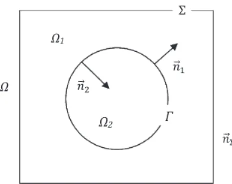
Letusconsideravolume

Ω

,boundedbyasurface

Σ

,anddefinedas

Ω

1U

Ω

2,wherethetwosubdomains

Ω

1 and

Ω

2

areseparatedbyaclosedsurface

Γ

with

Γ ∩ Σ = ∅

,asillustratedinFig. 1.Wedefinen

E

1 andn

E

2 asthenormalvectorsat

thesurface

Γ

pointingrespectivelytowards

Ω

1and

Ω

2.

Letusnowconsiderapiecewisecontinuousfunction

ψ

whichrespectsthePoissonequation,

1ψ =

0 (18)

insidebothsubdomains

Ω

1 and

Ω

2,withthefollowingjumpconditionattheinterface:

[ψ]

Γ

=

a

(E

xΓ

),

(19)

wherea

(E

xΓ

)

isafunctionoftheinterfacecoordinate

E

xΓ.Thejumpcondition(19)involvesthatthefollowingsurfaceintegral isequaltozero

Fig. 1.Sketch of a two-phase flow domainΩ1UΩ2with an immersed interfaceΓ.

¨

Γ

¡[ψ]

Γ

−

a

(E

xΓ

)¢E

n2dS

= E

0 (20)

Consideringa homogeneousDirichletboundaryconditionontheexternalboundary

Σ

ofthecomputationalfield,itcanbe easilydemonstratedthat

¨

Σ

ψ E

nΣdS

=

0

,

(21)

wheren

E

Σ isthenormalvectorpointingoutwardstheexternalboundary

Σ

.Thus

¨

Σ

ψ E

nΣdS

+

¨

Γ

¡[ψ]

Γ

−

a

(E

xΓ

)¢E

n2dS

=

0

.

(22)

Moreover,byremarkingthat

¨

Γ

¡[ψ]

Γ

−

a

(E

xΓ

)¢E

n2dS

=

¨

Γ

ψ E

n2dS

+

¨

Γ

ψ E

n1dS

−

¨

Γ a

(E

xΓ

)E

n2dS (23)

weobtainthefollowingequality:

¨

Σ

ψ E

nΣdS

+

¨

Γ

ψ E

n2dS

+

¨

Γ

ψ E

n1dS

=

¨

Γ a

(E

xΓ

)E

n2dS

.

(24)

Eq.(24)canalsobewrittenas

˚

Ω1

∇ψ

d

Ω +

˚

Ω2

∇ψ

d

Ω =

˚

Ω

∇ψ

d

Ω =

˚

Ω a

(E

xΓ

)E

n2

δ

Γd

Ω,

(25)

whichleadstothefollowinglocalformulation:

∇ψ =

a

(E

xΓ

)E

n2

δ

Γ

.

(26)

Finally,afterdifferentiation,weobtain:

1ψ = ∇ ·

¡

a

(E

xΓ

)E

n2

δ

Γ

¢.

(27)

Wehavethereforeshownthataddingthefollowingsourceterm

∇ · (

a

(E

xΓ

)E

n2

δ

Γ

)

totheright-handsideofaPoissonequation imposes a jump condition

[ψ]

Γ

=

a

(E

xΓ

)

onits solution

ψ

. Thisis alsovalid fora Poissonequation like eq. (18) witha right-handsidedifferentfromzero.

Moreover,followingasimilarapproach,itcanalsobedemonstratedthat ascalarfieldthatissolutionofthefollowing equation

1ψ =

b

(E

xΓ

)δ

Γ

,

(28)

withb

(E

xΓ

)

anotherfunctiondependingoninterfacecoordinate,willalsofulfillsthefollowingjumpcondition:

[E

n2

· ∇ψ] =

b

(E

xΓ

).

(29)

2.3. Projectionmethodfor whole-domainformulationand jump-conditionformulation

Letusconsidernowafirst-orderexplicitprojectionmethodforthesingle-phaseincompressibleNavier–Stokesequation. Itconsistsinprescribingafirstintermediate velocityfieldwhichdoesnotrespectthedivergence-freecondition(predictor step):

E

V₁∗

= E

Vn

− 1

t

¡¡

_E

Vn

· ∇

¢

_E

Vn

−

υ

1 E

Vn

− E

g

¢,

(30)

with

υ

thekinematicviscosity.

Next,aPoissonequationmustbesolvedtodeterminethepressurefield:

1

pn+1

=

ρ

n+1

∇ · E

V

∗

1

t

.

(31)

Then, in a last step, the final divergence-free velocity field can be computedusing the pressure field determined atthe previousstep:

E

Vn+1

= E

V∗

− 1

t

∇

p n+1

ρ

n+1

.

(32)

Applying the projection method toan incompressible two-phase flow isless straightforward. Dependingon whether the

whole-domainformulation orthejump-conditionformulation isused,theintermediatevelocityinthefirststepofthe

projec-tionmethodhastobedifferent.

Letusfirst considera whole-domainformulation. Anexplicit temporaldiscretizationof thecapillaryandviscous terms leadsquitenaturallytothefollowingpredictorstep

E

V₂∗

= E

Vn

− 1

t

µ

¡

_E

Vn

· ∇

¢

_E

Vn

−

∇ · (

2

µ

D n

₎

ρ

n+1

−

σ κ

n

E

δ

Γ

ρ

n+1

− E

g

¶

,

(33)

withthecorrespondingPoissonequation

∇ ·

µ

∇

pn+1

ρ

n+1

¶

=

∇ · E

V ∗ 2

1

t

= ∇ ·

µ

E

Vn

− 1

t

µ

¡

_E

Vn

· ∇

¢

_E

Vn

−

∇ · (

2

µ

D n

₎

ρ

n+1

−

σ κ

E

n

δ

Γ

ρ

n+1

− E

g

¶¶

.

(34)

Next,thecorrectionstepgives:

E

Vn+1

= E

V₂∗

− 1

t

∇

p n+1

ρ

n+1

.

(35)

Letusnowconsidertheapplicationoftheprojectionmethodtoajump-condition formulation oftheNavier–Stokesequation. Wehavetosolveeq.(5),sothefirststepoftheprojectionmethodissimilartoeq.(30)forasingle-phaseflow.Aswewant toimpose theappropriatejumpconditionattheinterfaceonthepressurefield (eq.(14)),we canshow,usingtheresults presentedinSection2.2,thatitcanbedone bysolvingthefollowingPoissonequation forthepressurewitharight-hand side splitintoacontinuouspartandasingularpart:

∇ ·

µ

∇

pn+1

ρ

n+1

¶

=

∇ · E

V ∗ 1

1

t

+ ∇ ·

µ (

σ κ

+

2

[

µ

]

Γ∂∂Vnn

)E

n

δ

Γ

ρ

n+1

¶

.

(36)

Using the splitting of the viscous term given ineq. (17)and notingthat n

E

·

D

· E

n

=

∂Vn

∂n , we find the following relation

betweenV

E

₂∗andV

E

₁∗:

E

V₂∗

= E

V₁∗

+ 1

t

(

σ κ

+

2

[

µ

]

Γ ∂Vn ∂n

)E

n

δ

Γ

ρ

n+1

.

(37)

Theuseofeq.(37)allowsdemonstratingthateq.(34)andeq.(36)areformallyidentical:

∇ ·

µ

_∇

_pn+1

ρ

n+1

¶

=

∇ · E

V ∗ 2

1

t

=

∇ · E

V₁∗

1

t

+ ∇ ·

µ (

σ κ

+

2

[

µ

]

Γ∂_∂V_nn

)E

n

δ

Γ

ρ

n+1

¶

.

(38)

Then,by consideringeq.(37),we candeducethefollowingcorrectionstepforajump-conditionformulation,leading tothe samefieldV

E

n+1 thanineq.(35):

E

Vn+1

= E

V₁∗

−

1

t

ρ

n+1

µ

∇

pn+1

−

µ

σ κ

+

2

[

µ

]

Γ

∂

Vn

∂

n

¶

E

n

δ

Γ

¶

.

(39)

To summarize,we have shownthatboth a whole-domainformulation and a jump-conditionformulation canbe used when applyinga projection methodtoan incompressibletwo-phaseflow. Thesetwo methodsare formally equivalent,butthey

leadtoadifferentdefinitionofthepredictedvelocityfield inthefirststepoftheprojectionmethod.In[10],the interme-diate velocity field V

E

₁∗ isused, whereas in[1,3,6,24] itis theintermediate velocity field V

E

₂∗.These twomethods will be respectivelynamedintherestofthispapertheGhost-FluidPrimitiveviscousMethod (GFPM)andtheDelta-FunctionMethod (DFM).

2.4.Projectionmethodforintermediateformulations

Other definitionsofthepredictedvelocityfieldarepossible.Forexample,weproposethefollowingtwo definitions,the respectiveinterestsofwhichwillbediscussedlater:

E

V₃∗

= E

Vn

− 1

t

µ

¡

_E

Vn

· ∇

¢

_E

Vn

−

∇ · (

2

µ

D n

₎

ρ

n+1

− E

g

¶

,

(40)

E

V₄∗

= E

Vn

− 1

t

µ

¡

_E

Vn

· ∇

¢

_E

Vn

−

∇ · (

µ

∇ E

V n

₎

ρ

n+1

− E

g

¶

.

(41)

Inthesamewayasintheprevious section,theyleadtothedefinitionofthesetwoPoissonequations,formallyequivalent toeq.(34)andeq.(36):

∇ ·

µ

_∇

_pn+1

ρ

n+1

¶

=

∇ · E

V ∗ 3

1

t

+ ∇ ·

µ

σ κ

n

E

δ

Γ

ρ

n+1

¶

,

(42)

∇ ·

µ

∇

pn+1

ρ

n+1

¶

=

∇ · E

V ∗ 4

1

t

+ ∇ ·

µ (

σ κ

+ [

µ

]

Γ∂_∂V_nn

)E

n

δ

Γ

ρ

n+1

¶

.

(43)

Thefollowingrelationshavebeenusedtodetermineeq.(43):

∇ · (

2

µ

D

) = ∇ ·

¡

µ

¡∇ E

V

+ ∇

T_V

_E

_{¢¢ = ∇ · (}

_µ

_{∇ E}

_V

_{) +}

_µ

_{∇ · ∇}

T_V

_E

_{+ ∇}

_µ

_{· ∇}

T_V

_E

_,

₍₄₄₎

∇ · (

2

µ

D

) = ∇ · (

µ

∇ E

V

) + [

µ

]

Γ

∇

TV

E

.E

n

δ

Γ

,

(45)

since

∇.∇

T_V

_E

₌

_{0 foranincompressibleflow,and}

E

n

.∇

TV

E

.E

n

=

∂

Vn

∂

n

.

(46)

Then,thetwofinalcorrectorsteps,respectivelysuitablewitheq.(40)andeq.(41),are:

E

Vn+1

= E

V₃∗

−

1

t

ρ

n+1

¡∇

p n+1

₋

_{σ κ}

_n

_E

_δ

Γ

¢,

(47)

E

Vn+1

= E

V₄∗

−

1

t

ρ

n+1

µ

∇

pn+1

−

µ

σ κ

+ [

µ

]

Γ

∂

Vn

∂

n

¶

E

n

δ

Γ

¶

.

(48)

The intermediate velocity field V

E

₃∗ hasalready been used inRefs. [5,21,26]in the framework of SharpInterfacemethods. Intherest ofthispaper,theGhost-FluidConservativeviscousMethod (GFCM)will referto thenumericalmethod proposed in[26].Finally, theuse of V

E

₄∗ leads to an original numericalmethod to deal withthe viscous terms,that we name the

Ghost-FluidSemi-ConservativeviscousMethod (GFSCM).

Thefourmethods DFM,GFPM,GFCMandGFSCM describedabove arethereforetheoretically equivalent,butthey lead to differentnumericalapproximations. The next objective ofthispaper isto discussabout their respectiveinterests and numericalaccuracy.

2.5.Spatialdiscretizationofsurfacetension

When a whole-domainformulation [3,6,12,24,30] is used, the surface-tension singular term isaccounted for when V

E

₂∗

iscomputed.The intermediatevelocity fieldisnext differentiatedto computetheright-hand sideofthepressurePoisson equation.Therefore,itiswellsuitedtoasmoothdiscretizationofthesurface-tensiontermthatinvolvesafictitiousinterface thickness. Its application to a sharp-interface description would be trickier. This approach is that of the Delta-Function

Method,known asContinuumSurfaceForce method.Inthisframework,thenumericaldiscretizationofdiscontinuousterms

makesuseofthefollowingregularizedsmoothedHeavisidefunctiondefinedfromtheLevel-Setfunction

φ

:

Hε

(φ) =











0 if

φ < −

ε

1 2

¡

1

+

φ_ε

+

sin( πφ ε ) π

¢

if

|φ| ≤

ε

1 if

φ > +

ε

,

(49)

where

ε

is the fictitious interface thickness, which is equal to 2 or 3 cell sizes. The surface-tension termcan then be computedusingthefollowingapproximation:

σ κ

n

E

δ

Γ

∼

=

σ κ

∇

Hε

.

(50) At the opposite, a projection method using a jump-conditionformulation with V

E

₁∗ as intermediate velocity field is well suitedforSharp-Interfacemethods.Thankstothisformulation, artificialsmoothingofinterfacesingularitiescanbe avoided, allowing a sharp-interface description.It has been used in the framework of Ghost-FluidMethod in [15], where authors propose afirst-orderdiscretization toimposea jumpconditiontothe solutionaswellastothe normalderivativeof the solutionwhensolvingthePoissonequation

∇ · (β∇

u

) =

f

,

(51)

i.e.withthefollowinginterfacejumpconditions

[

u

] =

a

(E

xΓ

)

and

·

β

∂

u

∂

n

¸

=

b

(E

xΓ

).

Consideringthatcapillaryeffectscanbe computedasajumpconditiononpressure,an originalSharp-Interfacemethod for solving the Navier–Stokesequation inthe framework ofLevel-Setmethods was introduced in[10].This methodhas been widely used to perform direct numericalsimulations oftwo-phase flows [16,26–29]. Letus now briefly summarize this approach.

Thediscretizationofa2DPoissonequationaseq.(51),whichinvolvesadiscontinuityofthesolutionandofitsnormal derivativeattheinterface,writes:

β

i+1/2 j

(

ui+1 j−ui j 1x

) − β

i−1/2 j

(

ui j−ui−1 j 1x

)

1

x

+

β

i j+1/2

(

ui j+1 −ui j 1y

) − β

i j−1 2

(

ui j−ui j−1 1y

)

1

y

=

fi j

+

gi j

+

hi j

,

(52)

whereinterpolations ofthediffusioncoefficient

β

onthecell bordersare computedastheharmonicaverage ofitsvalue

β

+ intheregion wherethe LevelSet functionis positiveandits value

β

− in theregion wheretheLevel Setfunction is negative;forexample,iftheinterfacecrossesameshsegmentbetweenxi andxi+1:

β

i+1/2 j

=

β

+

β

−

β

+

θ + β

−

(

1

− θ)

,

(53) with

θ =

|φ

i+1 j

|

|φ

i+1 j

| + |φ

i j

|

.

(54)

Thesourceterms gi j andhi j intheright-handsideofeq.(52)matchwiththediscontinuitiesofu andof

β

∂_∂un;theycanbe

computedas

gi j

=

gi jR

+

gi jL

+

gi jT

+

gBi j

,

(55)

hi j

=

hi jR

+

hLi j

+

hTi j

+

hi jB

,

(56)

whereeachofthesetermsarenon-zerowhenan interfacecrossesthecorrespondinggridsegment,andsuperscripts R,L,

T ,B denoterespectivelyright,left,topandbottomsides.Theirexpressionsare:

g_{i j}R

= ±

β

i+1/2 jaΓ

1

x2 g L i j

= ±

β

i−1/2 jaΓ

1

x2 g T i j

= ±

β

i j+1/2aΓ

1

y2 g B i j

= ±

β

i j+1/2 jaΓ

1

y2

,

(57) hR_{i j}

= ±

β

_i+1 2jbΓ

θ

β

±

1

x h L i j

= ∓

β

_i−1 2jbΓ

θ

β

±

1

x h T i j

= ±

β

_{i j+}1 2bΓ

θ

β

±

1

y h B i j

= ∓

β

_{i j−}1 2bΓ

θ

β

±

1

y

.

(58)

ItisnoteworthythatananalogycanbeestablishedbyusingtheresultsdemonstratedinSection 2.2andthediscretization described in thissection. Forsake ofsimplicity,let ustake a diffusioncoefficient

β

equal tounity. InSection 2.2,it has beenshownthatsolving

1

u

=

f with

[

u

] =

a

(E

xΓ

)

and

· ∂

u

∂

n

¸

=

b

(E

xΓ

)

isequivalenttosolve

1

u

=

f

+ ∇.

¡

a

(E

xΓ

)E

n

δ

Γ

¢ +

b

(E

xΓ

)δ

Γ

.

Comparingthisexpressionwithdiscreteequation(52),wededucethatsourceterms gi j andhi j,thatappearinthe

frame-workoftheGhost-FluidMethod,arerespectivelynumericalapproximationsof

∇.(

a

(E

xΓ

)E

n

δ

Γ

)|

i j andb

(E

xΓ

)δ

Γ

|

i j:

∇ · (

an

E

δ)|

i j

=

gi j

+

O

(1

x

)

(59)

b

δ|

i j

=

hi j

+

O

(1

x

)

(60)

Such ananalogyestablishesthelinkbetweentheContinuumSurfaceForce approachbasedonnumericalapproximationsof

2.6.Spatialdiscretizationofviscousterms

More details are provided in this section about the spatial discretization of viscous terms for the different methods described in the previous sections. In the following, for sake of simplicity, all developments are presented in 2D with Cartesiancoordinatesandauniformgrid.Thegeneralizationtoaxisymmetriccoordinatesor3Dgeometryisstraightforward.

2.6.1. Conservativeviscousformulation

Ifaconservativeviscousformulation

∇.(

2

µ

D)isconsidered,asitisthecaseintheGFCMorintheDFM,theprojection ofthedivergenceoftheviscous-stresstensorleadstothefollowingrelations:

∇ · (

2

µ

D

)|

x

=

∂

∂

x

µ

2

µ

∂

u

∂

x

¶

+

∂

∂

y

µ

µ

µ ∂

u

∂

y

+

∂

v

∂

x

¶¶

(61)

∇ · (

2

µ

D

)|

y

=

∂

∂

x

µ

µ

µ ∂

u

∂

y

+

∂

v

∂

x

¶¶

+

∂

∂

y

µ

2

µ

µ ∂

v

∂

y

¶¶

(62)

Letus remark that these two relations depend on both velocity components. This is whya fullyimplicit temporal dis-cretizationofviscoustermsismorecomplexwhenthisformulationisused.Suitableapproximationsofeq.(61)leadtothe followingspatialdiscretizations, Dx andDy denotingthedifferentialoperators:

¡∇ · (

2

µ

D

)¢ · E

ex

|

i+1/2 j

∼

=

Dx

(

2

µD

xu

)|

i+1/2 j

+

Dy

(

µD

yu

)|

i+1/2 j

+

Dy

(

µD

xv

)|

i+1/2 j (63) Dx

(

2

µD

xu

)|

i+1/2 j

=

2

µ

i+1 j

(

ui+3/2 j −ui+1/2 j 1x

) −

2

µ

i j

(

ui+1/2 j−ui−1/2 j 1x

)

1

x (64) Dy

(

µD

yu

)|

i+1/2 j

=

µ

i+1/2 j+1/2

(

ui+1/2 j+1 −ui+1/2 j 1y

) −

µ

i+1/2 j−1/2

(

ui+1/2 j −ui+1/2 j−1 1y

)

1

y (65) Dy

(

µD

xv

)|

i+1/2 j

=

µ

i+1/2 j+1/2

(

vi+1 j+1/2 −vi j+1/2 1x

) −

µ

i+1/2 j−1/2

(

vi+1 j−1/2 −vi j−1/2 1x

)

1

y (66)

Thefollowingspatialdiscretizationforeq.(62)is

¡∇ · (

2

µ

D

)¢ · E

ey

|

i j+1/2

∼

=

Dx

(

µD

yu

)|

i j+1/2

+

Dx

(

µD

xv

)|

i j+1/2

+

Dy

(

2

µD

yv

)|

i j+1/2 (67) Dx

(

µD

yu

)|

i j+1/2

=

µ

i+1/2 j+1/2

(

ui+1/2 j+1 −ui+1/2 j 1y

) −

µ

i−1/2 j+1/2

(

ui−1/2 j+1 −ui−1/2 j 1y

)

1

x (68) Dx

(

µD

xv

)|

i j+1/2

=

µ

i+1/2 j+1/2

(

vi+1 j+1/2 −vi j+1/2 1x

) −

µ

i−1/2 j+1/2

(

vi j+1/2 −vi−1 j+1/2 1x

)

1

x (69) Dy

(

2

µD

yv

)|

i j+1/2

=

2

µ

i j+1

(

vi j+3/2 −vi j+1/2 1y

) −

2

µ

i j

(

vi j+1/2−vi j−1/2 1y

)

1

y (70)

Thisspatial discretizationfortheconservativeviscous approachcan beusedboth intheframework ofSmoothed-Interface

methods (e.g.intheDFM)[3,24]orSharp-Interfacemethods (e.g.intheGFCM) [26].Thedifferenceliesinthewayviscosity

isapproximatedontheborderofacellthatiscrossedbyaninterface.

IntheDFM,eq.(8)isusedwiththeapproximationoftheHeavisidefunctiongivenbyeq.(49).

Inthe GFCMproposed by Sussmanetal.[26], theinterpolation usedto computeviscosity onthe cellborderis quite similar to that proposed by Liu et al.[15] to interpolate the diffusion coefficient of a Poisson equation (given here by eq.(53)).Thereafter,thiskindofinterpolationwillbeusedforallthecomputationsthatinvolvetheGhost-FluidMethod (i.e. GFCM,GFPMandGFSCM).

2.6.2. Ghost-FluidPrimitiveviscousMethod

TheGFPMofKangetal.[10] isnowbrieflydescribed. Whenthisapproachisused,thejump conditiononthenormal viscousstressesisaddedtothecapillaryforceswhensolvingthePoissonequationforpressureasshownineq.(36).

ThisapproachfortheviscoustermcanbesummarizedbyconsideringthefollowingprojectionsfortheLaplacianofthe velocity:

µ

1 E

V

|

x

=

µ

µ ∂

2_u

∂

x2

+

∂

2u

∂

y2

¶

,

(71)

µ

1 E

V

|

y

=

µ

µ ∂

2v

∂

x2

+

∂

2v

∂

y2

¶

.

(72)

(

µ

1 E

V

) · E

ex

|

i+1/2 j

∼

=

µ

¡

D2xu

|

i+1/2 j

+

D2yu

|

i+1/2 j

¢,

(73)

(

µ

1 E

V

) · E

ey

|

i j+1 2

∼

=

µ

¡

D2_xv

|

_{i j+}1 2

+

D 2 yv

|

i j+1 2

¢.

(74)

In[10],remarkingthatthevelocitygradientsarestronglydiscontinuousattheinterfacebecauseofviscosityjumps,itwas proposedtocomputeeachcomponentoftheLaplacianofthevelocity

µ

1 E

V (eqs.(73)and(74))bycomputingthedifferent termsofthevector

∇.(

µ

∇ E

V

)

andsubtractingtheirjumpattheinterface;onthex-axis,

µD

2xu

|

i+1/2 j

=

Dx

(

µD

xu

)|

i+1/2 j

− [

µD

xu

]δ

Γ

|

i+1/2 j

,

(75)

µD

2_yu

|

i+1/2 j

=

Dy

(

µD

yu

)|

i+1/2 j

− [

µD

yu

]δ

Γ

|

i+1/2 j

,

(76)

andonthe y-axis,

µD

2_xv

|

i j+1/2

=

Dx

(

µD

xv

)|

i j+1/2

− [

µD

xv

]δ

Γ

|

i j+1/2

,

(77)

µD

2_yv

|

i j+1/2

=

Dy

(

µD

yv

)|

i j+1/2

− [

µD

yv

]δ

Γ

|

i j+1/2

.

(78)

Theappropriatejumpconditionsforeqs.(75),(76),(77)and(78)aregiveninthefollowingmatrixby:

µ

[

_µ

∂u ∂x

] [

µ

∂u ∂y

]

[

µ

∂v ∂x

] [

µ

∂v ∂y

]

¶

= [

µ

]∇ E

V

µ

_E

0

E

t

¶

T

µ

_E

0

E

t

¶

+ [

µ

]E

nT

E

n

∇ E

Vn

E

Tn

E

− [

µ

]

µ

_E

0

E

t

¶

T

µ

_E

0

E

t

¶

∇ E

V

E

nTn

E

,

(79)

where

E

t istheunitvectortangenttotheinterface.

Tocomputeaccuratelyeqs.(75),(76),(77),(78)intheframeworkoftheGhost-FluidMethod[10],suitablesharp approxi-mations,eq.(58),oftheDiracdistributionarerequired.

Note that thejump conditionsineq. (79)are onlyvalid foracontinuous velocityfield betweenthe two phases:this approachcannotbeusedwhenphasechangesormasstransfersoccur.

2.6.3. GhostFluidSemi-ConservativeviscousMethod

IntheGFSCM,updatingV

E

₄∗ requirescomputingthefollowingviscousterms:

∇ · (

µ

∇ E

V

)|

x

=

∂

∂

x

µ

µ

∂

u

∂

x

¶

+

∂

∂

y

µ

µ

∂

u

∂

y

¶

,

(80)

∇ · (

µ

∇ E

V

)|

y

=

∂

∂

x

µ

µ

∂

v

∂

x

¶

+

∂

∂

y

µ

µ

∂

v

∂

y

¶

.

(81)

Thatcanbedone inasimilarway asfortheconservativeviscous approach,exceptforthesecond-ordercross-derivatives, which are non-zeroonly atthe interface andare therefore includedin thepressure jump whenthe Poissonequation is solved.As pointedout previously,thisapproachcanbeusedwithanimplicittemporaldiscretizationoftheviscousterms andalsowhenaphasechangeoccurs.

2.7. Implicittemporaldiscretizationofviscousterms

Furtherelementsareprovidednowtodealwithanimplicittemporaldiscretizationofviscousterms.

When theincompressibleNavier–Stokesequationsforasingle-phasefloware considered,theprojection methodleads tothefollowingsemi-implicitalgorithmforthepredictorstep

E

V₁∗

− 1

tυ

1 E

V₁∗

= E

Vn

− 1

t

¡

_E

Vn

· ∇

¢

_E

Vn

,

(82)

whichrequiressolvinganindependentlinearsystemforeachvelocitycomponent.

When atwo-phase flow witha discontinuousviscosity isconsidered, theuseofa semi-implicitprojection methodto solvetheincompressibleNavier–Stokesequationsismorecomplex.Indeed,in2D,thefollowingtwo coupledequationsmust besolvedsimultaneously,leadingtoamorecomplicatedlinearsystemasitiscarriedoutin[25,26]:

ρ

n_i++₁1_{/2 j}u∗_{i+1/2 j}

− 1

t

¡

Dx

¡

2

µD

xu∗

¢ +

Dy

¡

µD

yu∗

¢ +

Dy

¡

µD

xv∗

¢¢¯

¯

i+1/2 j

=

ρ

_in₊+₁1_{/2 j}

¡

un_{i+1/2 j}

− 1

t

¡

_E

Vn

· ∇

¢

un

|

i+1/2 j

¢,

(83)

ρ

n_{i j}+₊1_1/2v∗_{i j+1/2}

− 1

t

¡

Dx

¡

µD

yu∗

¢ +

Dx

¡

µD

xv∗

¢ +

Dy

¡

2

µD

yv∗

¢¢¯

¯

i j+1/2

=

ρ

_{i j}n+₊1_1/2

¡

vn_{i j+1/2}

− 1

t

¡

_E

Vn

· ∇

¢

vn

|

i j+1/2

¢.

(84)

ρ

_in₊+₁1_{/2 j}u∗_{i+1/2 j}

− 1

t

¡

Dx

¡

2

µD

xu∗

¢ +

Dy

¡

µD

yu∗

¢¢¯

¯

i+1/2 j

=

ρ

n_i++11/2 j

¡

un_{i+1/2 j}

− 1

t

¡

_E

Vn

· ∇

¢

un

¯

¯

i+1/2 j

¢ + 1

t Dy

¡

µD

xvn

¢¯

¯

i+1/2 j

,

(85)

ρ

_{i j}n+₊1_1/2v∗_{i j+1/2}

− 1

t

¡

Dx

¡

µD

xv∗

¢ +

Dy

¡

2

µD

yv∗

¢¢¯

¯

i j+1/2

=

ρ

n_{i j}+₊1_1/2

¡

vn_{i j+1/2}

− 1

t

¡

_E

Vn

· ∇

¢

vn

¯

¯

i j+1/2

¢ + 1

t Dx

¡

µD

yun

¢¯

¯

i j+1/2

.

(86)

Nevertheless,itisdoubtfulthatthenumericalschemecomposedofeqs.(85),(86)reallyalleviatesthetimestepconstraint imposedbyviscositysincethelasttermsontherightistreatedexplicitly.

Anotherway tocarry outanimplicittreatmentoftheviscous termsforincompressibleflowsisproposed in[11].This isbasedonanapproximatefactorizationwhichrequiressolvingtridiagonalmatricesratherthaninversionofalargesparse matrix.Thisalternativemethodhasnotbeentestedinthiswork.

Attheopposite,asithasbeenpreviouslyshown,forincompressibleflowsthesecond-ordercross-derivativesareperfectly compensatedeverywhereexceptattheinterfacewhereviscosityisdiscontinuous. Therefore,theGFSCMcanbe usedwith benefitswithanimplicittreatmentoftheviscousterms,whichleadstothefollowingdiscretization:

ρ

_in₊+₁1_{/2 j}u∗_{i+1/2 j}

− 1

t

¡

Dx

¡

µD

xu∗

¢ +

Dy

¡

µD

yu∗

¢¢¯

¯

_{i+1/2 j}

=

ρ

n_i++₁1_{/2 j}

¡

un_{i+1/2 j}

− 1

t

¡

_E

Vn

· ∇

¢

un

|

i+1/2 j

¢,

(87)

ρ

_{i j}n+₊1_1/2v∗_{i j+1/2}

− 1

t

¡

Dx

¡

µD

xv∗

¢ +

Dy

¡

µD

yv∗

¢¢¯

¯

i j+1/2

=

ρ

n_{i j}+₊1_1/2

¡

vn_{i j+1/2}

− 1

t

¡

E

Vn

· ∇

¢

vn

|

i j+1/2

¢.

(88)

Theresultinglinearsystemscanbesolvedaseasilyasinthesingle-phasecase:thematricesofdiscretizationaresymmetric, definite and positive, which allows the use of an efficient andsimple black-box solver. Note that an implicit temporal discretizationoftheviscoustermscanalsobeusedwiththeGFPM[8].

Weconcludebysomecommentsonthewaytodefinethedensity:

ρ

n_i++₁1_{/2 j} and

ρ

_{i j}n+₊1_1/2.Thedefinitionmustbe compat-iblewiththecomputation ofthecorrectionstep,whichitselfreliesonthemannerdensityiscomputedwhenthePoisson equation on pressure is solved. Accurate resultsare obtainedby using the following generalexpression for

ρ

n_i++₁1_{/2 j} and

ρ

n_{i j}+₊1_1/2 inthegridcellsthatarecrossedbyaninterface:

1

ρ

n+1

=

1 ρ+_ρ− 1 ρ+

θ +

_ρ1−

(

1

− θ)

=

1

ρ

−

_{θ +}

_ρ

+

₍

₁

_{− θ)}

.

(89)

2.8.Summaryaboutthefourdifferentmethodstodealwithviscosity

Table 1givesanoverviewofthecharacteristicsofthefourdifferentmethodstodealwithviscoustermsinthe simula-tionsoftwo-phaseflowswithLevel-Setmethods,anddescribesthemainstepsforimplementingit.

2.9. Level-Setmethodsforinterfacecapturing

Interfacemotion is capturedwith a Level-Setmethod [20,24], which consistsin solving a convection equation forthe Level-Setfunction

φ

:

∂φ

∂

t

+ ( E

V

· ∇)φ =

0

,

(90)

withV the

E

velocityattheinterface.Areinitializationstep[24]cannextbeperformedtoinsurethatthe

φ

functionremains

asigneddistanceinthecomputationdomain.ThiscanbedonebysolvingiterativelythespecificPDE:

∂

d

∂

τ

=

sign

(φ)

¡

1

− |∇

d

|¢,

(91)

whered isthe reinitialized distancefunction,

τ

a fictitiousreinitialization time andsign(

φ

) asmoothed signed function definedin [4,24].At the endof every physicaltime step, two temporal iterations of the redistancing equation (91) are solvedusingasecond-orderTVD–Runge–Kuttascheme.

Thesigneddistancefunctionallowspreservingagoodaccuracywhencomputinginterfacegeometricalpropertiesasthe normalvectororthecurvaturewiththefollowingsimplerelations:

E

n

=

∇φ

|∇φ|

,

(92)

Table 1

SummaryoffourdifferentmethodstodealwithviscoustermswithLevel-Setmethods.

Framework Methodandreferencepapers Stepsoftheexplicitprojectionmethodandnumber ofthe correspondingequationsinthereferencepaper

Implementationofan implicitmethod “Wholedomain formulation” Delta-FunctionMethod DFM Sussmanet al.[3,24,25] E V∗ 2= EVn− 1t¡( EVn· ∇) EVn− ∇·(2µDn₎ ρn+1 −σ κ E nδΓ ρn+1 − Eg ¢

(33) Onecomplexcoupled paraboliclinearsystemfor allthevelocitycomponents

∇ ·¡∇pn+1 ρn+1 ¢ = ∇· EV∗ 2 1t (34) E Vn+1_{= EV}∗ 2− 1t ∇pn+1 ρn+1 (35) “Jumpcondition formulation”

Ghost-FluidPrimitiveviscous Method GFPM Kangetal.[10] Hongetal.[8] E V∗ 1= EV n_{− 1t¡( EV}n_{· ∇) EV}n₋µ1 EVn ρn+1 − Eg ¢

(30) Severalsimpleindependent linearsystemswithexplicit jumpconditionsonthe componentsoftheviscous tensor ∇ ·¡∇pn+1 ρn+1 ¢ = ∇· EV∗ 1 1t + ∇ · ¡(σ κ+2[µ]Γ∂∂Vnn)EnδΓ ρn+1 ¢ (36) ⇔    ∇ ·¡∇pn+1 ρn+1 ¢ = ∇· EV∗ 1 1t [pn+1_] Γ=σ κ+2[µ]Γ∂∂Vnn E Vn+1_{= EV}∗ 1− 1t ρn+1¡∇p n+1₋¡ σ κ+2[µ]Γ∂∂Vnn¢EnδΓ¢ (39) Ghost-FluidConservative viscousMethod GFCM Sussmanet al.[26] E V∗ 3= EV n_{− 1t¡( EV}n_{· ∇) EV}n₋∇·(2µDn) ρn+1 − Eg ¢

(40) Onecomplexcoupled paraboliclinearsystemfor allthevelocitycomponents

∇ ·¡∇pn+1 ρn+1 ¢ = ∇· EV∗ 3 1t + ∇ · ¡σ κ EnδΓ ρn+1 ¢ (42) ⇔ ( ∇ ·¡∇pn+1 ρn+1 ¢ = ∇· EV∗ 3 1t [pn+1_] Γ=σ κ E Vn+1_{= EV}∗ 3− 1 t ρn+1(∇pn+1−σ κnEδΓ) (47) Ghost-Fluid Semi-Conservativeviscous Method GFSCM Presentpaper E V∗₄= EVn_{− 1t¡( EV}n_{· ∇) EV}n₋∇·(µ∇ EVn₎ ρn+1 − Eg ¢

(41) Severalsimpleindependent linearsystemswithoutany jumpconditionsonthe componentsoftheviscous tensor ∇ ·¡∇pn+1 ρn+1 ¢ = ∇· EV∗ 4 1t + ∇ · ¡(σ κ+[µ]Γ∂∂Vnn)EnδΓ ρn+1 ¢ (43) ⇔    ∇ ·¡∇pn+1 ρn+1 ¢ = ∇· EV∗ 4 1t [pn+1_] Γ=σ κ+ [µ]Γ∂∂Vnn E Vn+1_{= EV}∗ 4−ρ1n+t1¡∇pn+1− ¡ σ κ+ [µ]Γ∂∂Vnn¢EnδΓ¢ (48)

The curvature is firstly computed on all the grid nodes with simple finite difference schemes. Next,if the Ghost Fluid Methodisused,thecurvatureisinterpolatedontheinterface.Forexample,ifitcrossesthesegment

[

x_i

,

x_i+1

]

thefollowing

interpolationisused:

κ

I

=

κ

i+1

θ +

κ

i

(

1

− θ)

(94)

2.10. Temporalandspatialdiscretizations

Allconvective termsandspatial derivativesoftheredistanceequationare discretizedbymeansofa fifth-orderWENO 5scheme[9].First-orderexplicitorsemi-implicittemporalintegrationmethodshavebeendescribed inprevioussections. Theseelementarystepsarefinallyincludedinasecond-orderTVD–Runge–Kutta schemefortheoveralltemporalintegration of the PDE systemin order to improve the computation stability. A classical time-step constraint [10,23,24] accounting for thestability conditions onconvection, viscosity(in caseof an explicittemporal discretization) andsurface tensionis imposed.

1

tconv

=

1

x max

k E

V

k

(95)

1

tvisc

=

1 4

1

x2

max

(

υ

liq

,

υ

gaz

)

(96)

1

tsurf_tens

=

1 2

s

ρ

liq

1

x3

σ

(97)

Ifan implicittemporaldiscretizationisusedwiththeGFSCM,an explicitpartdependingon theviscosityjumpcondition remains inEqs.(43),(48).Therefore,thecorresponding terminvolvesanothertemporalconstraintwhichisdifferentfrom Eq.(96),since it dependsona viscosity jumpconditioninstead ofa maximumkinematicviscosity value. Byperforming several numericaltest-cases withzero surface tensionand verylow gravity(in order to remove the stability constraints duetosurfacetensionandconvection),wehaveobservedthatthefollowingtimesteprestrictionissufficienttoensurethe numericalstability:

1

tvisc

=

ρ

1

x2

[

µ

]

(98)

with

ρ

theaveragedensityofthetwophases.Whereasthisconstraintdependsalsoon

1

x2_{,itcanbemuchmorelenient}

thanthe classical one,Eq. (96), because _[µρ_]

∼

1

υliq is muchhigherthan

1

υgas formanytypical gas–liquidsystems suchas

air–waterortheoneusedin Section3.3.Forexample,itisshownin Section3.3thattheimplicitGFSCMallowsperforming thecomputationwithamuchlargertimestepincomparisontoitsexplicitcounterparts.

Finally,theglobaltimesteprestrictioncanbecomputedwiththefollowingrelation:

1

1

t

=

1

1

tconv

+

1

1

tvisc

+

1

1

tsurf_tens (99) 3. Numericalresults

Relevantbenchmarkshavebeendesignedtoassessandcomparethefourdifferentnumericalmethodsdiscussedinthis paper:DFM,GFPM,GFCMandGFSCM.

Inthefirstbenchmark,computationsofa sphericalbubblerisingundergravity areperformedforarangeofReynolds numbervaryingfrom20to100.

The second benchmark consistsof numerical simulations ofbubble shape-oscillations in the absenceof gravity. Such a physicalproblemis characterized by an oscillationReynolds numberwhichcompares the oscillations frequencyto the dampingrate. The accuracy of thesimulations is evaluated fromcomparisons withthe theoretical prediction ofthe fre-quencyandthedampingrateoftheoscillationsforReynoldsnumbersvaryingfrom20to300. Inaddition,a studyofthe spatialconvergenceofthesimulations iscarriedoutinordertodeterminehowmesh-gridrequirementsevolve whenthe Reynoldsnumberisvaried.

Finally,thethirdbenchmarkfocusesontheriseofanon-sphericalbubbleinaveryviscousliquidasinRefs.[2,6,26]. Thesethreebenchmarksconsistofaxisymmetriccomputations.

3.1. Asphericalbubblerisingundergravity

Currently,performingwell-resolvedsimulationsofbubblyflowsordropletspraysisachallengeforthedirectnumerical simulationoftwo-phase flows.Manyissuesmustbe overcometoachieve suchambitioustargets.Onecanexpect thatthe developmentofHighPerformanceComputinghardwareandsoftwarewillallowperformingsimulationsinvolvingagrowing numberofbubblesordrops.Howeverwell-resolved3Dsimulationsremaincostlyandaparticularattentionmustbepaidto thedevelopmentandtheassessmentofaccuratenumericalmethodstosolvethefluiddynamicsequations.Inparticular,a computationwhichisefficienttodescribeaccuratelythedynamicswithhalfthenumberofgridcellsonabubblediameter makespossibletocomputeeighttimesmorebubbleswiththesamecomputationalresources.Actually,thegainwouldeven besignificantlygreatersince,forexplicitmethods,alargertimestepcanbeused onacoarsergrid.Thetest-caseproposed inthis section allows us to assessthe different discretizations of theviscous terms.Simulations are performedwithan axisymmetriccoordinatesystem.Theradialandaxialsizesofthecomputationaldomainaredefinedrelativelytothebubble radiusRbubble:lr

=

8Rbubbleandlz

=

4lr.Consideringasphericalbubble,referenceresultsonthedragcoefficientareprovided

byboundary-fittednumericalsimulationsfrom[19]whenRe∞

≤

50 orbyMoore’stheory[18]forhigherReynoldsnumbers. OurcomputationsareperformedforlowBondnumberstopreservebubblesphericity.Itisworthmentioningthatthecase ofarisingsphericalbubbleisparticularlyadvisedtoassessthediscretizationoftheviscoustermsbecause,inthissituation, thedrag forcemainly dependsonviscousdissipation andnoton pressureeffects,unlike thecaseofastronglydeformed bubble.

Thephysicalpropertiesofliquidandgasarekeptidenticaltowaterandairforallsimulationspresentedinthissection:

ρ

liq

=

1000 kg m−3,

µ

liq

=

0

.

00113 kg m−1s−1,

ρ

gas

=

1

.

226 kg m−3,

µ

gas

=

1

.

78

×

10−5 kg m−1s−1.Simulationconditions

aresummarizedinTable 2forfiveconfigurationscorrespondingtoRe∞

=

20,40,60foraBondnumberBo

=

0

.

025,andto Re∞

=

80

,

100 forBo

=

0

.

0125.Bubbles areinitiallystaticandevolve undergravityuntiltheterminalvelocity isreached. Theboundariesofthecomputationaldomainaredefinedaswalls(except onsymmetryaxis)andsetsufficientlyfarfrom thebubbletohaveanegligibleinfluenceontheresults.

Simulationsareperformedwiththreedifferentmeshgrids(32

×

128,64

×

256,128

×

512,256

×

1024),whichdescribe respectivelyonebubblediameterwith8,16,32or64meshpoints.Fig. 2showsasnapshotoftheinterfacelocationandthe fully-developedvorticityintheframemovingwiththe bubbleforthecaseRe∞

=

60 with thethinnestgrid.Resultsofall thesimulationsaresummarizedinTables 3,4,5,6 and7,whichcorrespondrespectivelytocomputationscarriedoutusing

theGhostFluidConservativeviscousMethod (GFCM),explicitandimplicitGhost-FluidSemi-ConservativeviscousMethod (GFSCM),

Ghost-FluidPrimitiveviscousMethod (GFPM)andDelta-FunctionMethod (DFM).Many conclusionscan be drawnfromthese

tables.First,allmethodsfailtoprovideaccurateresultsonthecoarsestgridregardlessthevalueofRe∞:thismeshisclearly insufficienttocaptureaccuratelyviscouseffects.Whentheintermediategridisused,theGFCMandtheexplicitandimplicit GFSCMprovidesverygoodresults:whateverRe∞,deviationsbetweenreferenceresultsandnumericalsimulationsareless orequalto3% (exceptforRe∞

=

80 whentheexplicitGFSCMisused).TheGFPMalsoprovidesacceptable resultsonthis

Table 2

Bubbleradius,gravityacceleration,surfacetensionandfinaltimeofsimulationforasphericalbubblerisingat variousReynoldsnumbers.

Re∞=20 Re∞=40 Re∞=60 Re∞=80 Re∞=100

Rbubble(µm) 19.55 44.65 70.45 98.95 127.9

gz(m s−2) −9144.4 −1755.2 −705.6 −357.5 −213.9

σ(N m−1_{) 0.56 0.56 0.56 1.12 1.12}

tf (s) 0.0004 0.00135 0.002375 0.0048 0.007

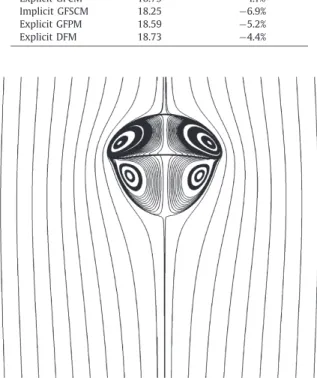
Fig. 2.Streamlines,interfacelocationandvorticityfield(s−1_{)inthemovingframeofarisingsphericalbubbleatRe}

∞=60 (grid128×512)usingthe

GFCM.

Table 3

ErrorontheterminalReynoldsnumberofrisingbubblesfordifferentcomputationalgridswiththeexplicitGFCM. Grids Re∞=20 Re∞=40 Re∞=60 Re∞=80 Re∞=100 32×128 −22.0% −34.0% −38.8% −63.0% −67.4% 64×256 +2.5% +1.8% −1.3% −1.3% −3.0% 128×51 +0.5% +0.8% −1.0% +1.9% +1.9% 256×1024 −0.9% −0.4% −1.95% −1.02% −0.65% Table 4

Error onthe terminalReynoldsnumber ofrisingbubbles for differentcomputationalgridswith the explicit GFSCM. Grids Re∞=20 Re∞=40 Re∞=60 Re∞=80 Re∞=100 32×128 −23.5% −32.5% −39.0% −62.5% −67.0% 64×256 −0.5% +2.5% +1.3% +4.3% +3.0% 128×512 −3.5% +0.6% 0.7% +5.4% +6% 256×1024 −2.15% +3.25% +4.2% +6.75% +8.2% Table 5

Erroron theterminalReynoldsnumberofrisingbubblesfor differentcomputationalgridswith theimplicit GFSCM. Grids Re∞=20 Re∞=40 Re∞=60 Re∞=80 Re∞=100 32×128 −18.6% −25.0% −30.2% −52.9% −55.1% 64×256 −1.2% 1.5% −0.1% 2.0% 0.9% 128×512 −3.7% 0.1% −0.2% 3.2% 3.9% 256×1024 −4.2% 3% 4% 6.25% 7.6%

Table 6

ErrorontheterminalReynoldsnumberofrisingbubblesfordifferentcomputationalgridswiththeexplicitGFPM. Grids Re∞=20 Re∞=40 Re∞=60 Re∞=80 Re∞=100 32×128 −16.7% −24.6% −31.5% −52.3% −56.8% 64×256 0.5% −1.2% −4.5% −4.8% −6.6% 128×512 0.1% −0.3% −2.6% −1.0% −1.6% 256×1024 −0.7% −0.67 −2.6% −1.3% −1.4% Table 7

ErrorontheterminalReynoldsnumberofrisingbubblesfordifferentcomputationalgridswiththeexplicitDFM. Grids Re∞=20 Re∞=40 Re∞=60 Re∞=80 Re∞=100

32×128 −39.5% −46.1% −53.8% −75.8% −81.6% 64×256 −16.5% −18.3% −21.7% −29.3% −31.8% 128×512 −7.5% −7.9% −9.9% −10.5% −10.9% 256×1024 −4.3% −4.65% −6.6% −6.04% −6.05%

gridsincethediscrepancybetweennumericalsimulationsandreferencesolutionsisless than7%;theerrorincreaseswith theReynoldsnumber,whichisprobablyduetothedifficultytocalculateaccurately boundarylayersthat becomesthinner athighRe∞.Bycontrast,theDFMprovidesaloweraccuracythantheothermethodswitherrorsonRe∞ whichvaryfrom 15%to30%andincreasewithRe∞.Finally,consideringresultsobtainedwiththemostrefinedgrids,itclearlyappearsthat boththeGFCMandtheGFPMhaveconvergedtothecorrectsolution.TheexplicitandimplicitGFSCMprovideresultswith largererrorsthan thetwoprevious methodswitherrorsvarying between2% and8%. TheDFMseems toconvergeslowly towardsthetheoreticalsolutionandstill showsdeviationsvaryingfrom4%to6%(accordingtoRe∞)with64meshpoints onabubblediameter.

3.2.Shapeoscillationsofabubble

Consideringsmall-amplitude-shape-oscillations ofa bubblein the absence of gravity, theoretical solutions ofthe lin-earizedNavier–Stokesequationsforanincompressibleflowexistandgiveexpressions forthe frequencyandthedamping rateof the oscillations [17,22]. We have took advantage of this to design an accurate and stringent test-casefor direct numerical simulations. While the oscillation frequency depends essentially on capillary effects, we have focused on the damping ratein order to test the accuracy of different numerical approachesabout viscosity. Like in the previous sec-tion,simulations are performedwithan axisymmetric coordinateframe. The dimensions ofthe computational field are: lr

=

4Rbubble,lz

=

2lr.Wallboundaryconditionsareusedonalldomainborders(exceptonsymmetryaxis)andconfinement

effectshavebeencheckedtobenegligible.Densitiesandviscosities,correspondingtoanair/watersystem,arethesameas inSection3.2,andthesurfacetensionis

σ

=

0

.

07 N m−1_{.WeproposeaparametricstudybyvaryingtheReynoldsnumber}

ofoscillation,by Reosc

=

p

σRbubbleρliq

µliq ,from20 to300. (Note that theReynoldsnumberof oscillationisthe inverseofthe

Ohnesorgenumber.)

Inoursimulations,theinitialconditioncorrespondstoadeformedinterfacedescribedbyaLegendrepolynomialoforder 2withthefollowingLevelSetfunction

φ (

r

, θ,

t

=

0

) =

r

−

Rbubble

£

1

+

ε

P2

(

cos

θ )¤,

(100)

where

(

r

,

θ )

are thesphericalcoordinates, P2

(

cos

θ )

=

₂1

(

3cos2

θ −

1

)

and

ǫ

isthedimensionlessinitial amplitudeofthe

deformation,chosenlow enough(

ε

=

0

.

075)tomaintaintheoscillationsinthelinearregime.Thecomputedshapeofthe interfaceisextractedateachtimestepanddecomposedintosphericalharmonicsinordertoobtainthetimeevolutionof amplitudea₂

(

t

)

ofharmonicl

=

2:

r

(θ,

t

) =

Rbubble

+

a2

(

t

)

P2

(

cos

θ ).

(101)

Then,thefrequency

ω

2 andthedampingrate

β

2 oftheoscillationsareobtainedfroma2

(

t

)

since

a2

(

t

) =

εR

bubblecos

(

ω

2t

)

e−β2t (102)

Thevaluesissuedfromthesimulationsarecomparedwiththetheoreticalvalues

ω

th₂ and

β

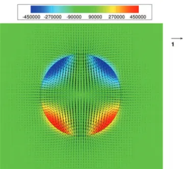
₂ththatarecomputedbysolving numericallythecharacteristicequation givenby Prosperetti(eq.(33)ofRef.[22]).Thedampingrateisaglobalparameter thatrequiresanaccuratecalculationoftheviscoustermsalloverthecomputationdomain.

Snapshotsofthe interfacelocation andvorticity areshowninFig. 3andFig. 4forReosc

=

20 andReosc

=

200,

respec-tively.It is clearfrom thesefigures that the vorticity islocalized inside the bubble,whereas theflow remains potential outside.Forashape-oscillatingbubble,boththefrequencyandthedampingratearemainlycontrolledbythepotentialflow inthe liquidphase.The asymptoticdevelopment of thedampingrate givenby MillerandScriven [17] showsthat, fora bubble,theviscousdissipation intheboundarylayers isresponsibleforonly1to3% ofthetotaldissipation inapresent

Fig. 3.Velocity field, interface location and vorticity field (s−1_{) of an oscillating bubble at Re}

osc=20 (grid 256×512) using the GFCM.

Fig. 4.Velocity field (m s−1_{), interface location and vorticity field (s}−1_{) of an oscillating bubble at Re}

osc=200 (grid 256×512) using the GFCM.

Table 8

Erroronthedampingrateβ2foranoscillatingbubblewithdifferentcomputationalgridswiththeexplicitGFCM.

Grids Reosc=20 Reosc=50 Reosc=100 Reosc=200 Reosc=300

64×128 1.49% 1.47% 9.75% 23.16% 41.72% 128×256 −0.20% 0.32% 1.99% 7.30% 13.71% 256×512 −0.31% 0.08% 0.70% 2.55% 5.36%

range of Reosc, i.e. between 20and 300. The restof the viscous dissipation comes fromthe potential flow in the liquid

phase.

ForeachReynoldsnumberofoscillation,atesthasbeencomputedwithfourdifferentnumericalmethods(GFCM,explicit GFSCM,GFPMandDFM)andforthreedifferentmeshgrids

(

64

×

128

)

,

(

128

×

256

)

and

(

256

×

512

)

,whichdescribeabubble diameterwith32,64and128meshpoints,respectively.TheresultsofthesimulationsaresummarizedinTables 8,9,10 and 11,wherethedeviationofthenumericalsimulationsrelativetothe theoreticalpredictionshavebeenreported.The error on thefrequencyofoscillation isverysmall (

<

1%)whateverthenumericalmethod andthemeshgrids;it hastherefore

Table 9

Erroronthedampingrateβ2foranoscillatingbubblewithdifferentcomputationalgridswiththeexplicitGFSCM.

Grids Reosc=20 Reosc=50 Reosc=100 Reosc=200 Reosc=300

64×128 −4.57% −7.16% −0.30% 13.06% 31.04% 128×256 −3.90% −7.58% −6.47% 0.38% 8.78% 256×512 −2.69% −7.52% −12.13% −4.21% −0.77%

Table 10

Erroronthedampingrateβ2foranoscillatingbubblewithdifferentcomputationalgridswiththeexplicitGFPM.

Grids Reosc=20 Reosc=50 Reosc=100 Reosc=200 Reosc=300

64×128 2.88% 3.11% 10.39% 22.34% 39.62% 128×256 0.23% 0.68% 1.66% 5.90% 11.70% 256×512 −0.10% −0.00% −1.04% 1.31% 3.52%

Table 11

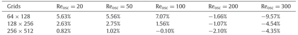
Erroronthedampingrateβ2foranoscillatingbubblewithdifferentcomputationalgridswiththeexplicitDFM.

Grids Reosc=20 Reosc=50 Reosc=100 Reosc=200 Reosc=300

64×128 5.63% 5.56% 7.07% −1.66% −9.57% 128×256 2.63% 2.75% 1.56% −1.07% −4.54% 256×512 0.82% 1.02% −0.10% −2.10% −4.35%

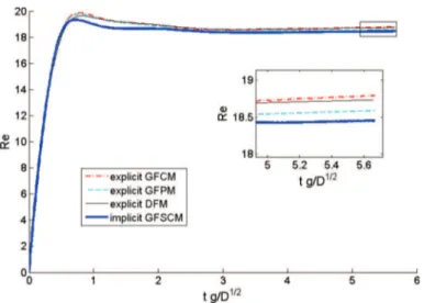
Fig. 5.Temporalevolutionofamplitudeofmode2atReosc=100.Comparisonsbetweentheory(fromRef.[20])andnumericalsimulationswiththeGFCM

andtheGFSCM.Timeisnormalizedbythetheoreticalperiodofoscillationofmode2,T₂th.

notbeenreported.Adetailedanalysisoftheerrorsonthedampingrateleadstothefollowingconclusions.First,theGFCM andthe GFPM accurately matchwiththe exactsolution when refined grids are used.Both methods presentcomparable abilitieson this test-case, witherrors less than 2% in therange 20

≤

Reosc

≤

200 (the GFPM is just slightly better than

theGFCM).ForthehighestReynoldsnumbersofoscillationconsidered,theerrorseemstodecreasemonotonouslyandthe orderofconvergencecanberoughly estimatedto 1.5.Thatisnotsurprisingconsideringthat,even ifthediscretizationof viscous termsremains ofthe second orderfar fromtheinterface, the subcellviscosityinterpolation inthe cells thatare crossedby aninterface isonlyofthefirstorder.The DFMalsoprovides goodresultsinthiscaseandconvergeswell,but exhibitsadifferentbehavior thantheGFCMortheGFPM.Forexample,whencoarsegridsareused,theerrorisrelatively low(between5and10%)whatevertheReosc,contrarytothetwopreviousmethodswheretheerrorwasclearlyincreasing

withReosc tobecome largerthan20% atthehighestReosc.The rateofconvergenceof theDFMisnot asclearasforthe

GFCMortheGFPM.Finally,theexplicitGFSCMprovidespoorresultswitherrorsupto12%insomecaseswiththethinnest grid.Althoughthisdiscrepancyisnotnegligible,amoredetailedanalysisofthetemporalsignala2

(

t

)

,presentedinFig. 5for

themostdisadvantageouscasefortheGFSCM(Reosc

=

100,grid256

×

512),allowsustorealizethatthisunderestimation

of12%ofthedampingratedoesnotinduceasosignificantdifferencecomparedtotheothermethods.

Inaddition,itisworth mentioningthattheGFCMhasbeensuccessfullyusedinRef.[13] tosimulate theshape oscilla-tionsofrisingdropsandbubbles inordertodeterminetheeffectoftherising motiononthefrequencyandthedamping rateoftheoscillations.