Do habitat measurements in the vicinity of Atlantic salmon (Salmo salar) parr matter? 1
2 3
Julien MOCQ a, b†, André ST-HILAIRE c, d and Rick A. CUNJAK d 4
a
Department of Ecosystems Ecology, Faculty of Science, University of South Bohemia, 5
Branisovska 31, CZ-37005 Ceske Budejovice, Czech Republic 6
b
Biology Centre AS CR, Institute of Entomology, Laboratory of Aquatic Insects and Relict 7
Ecosystems, Branisovska 31, CZ-37005 Ceske Budejovice, Czech Republic 8
c
INRS-ETE, Université du Québec, 490 rue de la Couronne, Québec, QC, G1K9A9, Canada. 9
d
Canadian River Institute, Department of Biology, University of New-Brunswick, P.O. Box 10
4400, Fredericton, NB, E3B5A3, Canada 11
† Corresponding author (e-mail: jmocq@prf.jcu.cz; Tel: +420 774 537 779) 12
13 14
Submitted to: 15
Fisheries Management and Ecology 16
17 18
Abstract 19
Atlantic salmon (Salmo salar) parr habitat characterization is usually performed by in situ 20
measures of key environmental variables, taken at the exact fish location, or conversely, in large 21
sampling sections, often ignoring variability in the immediate vicinity around individuals. These 22
data may have a critical importance in development and validation of habitat preference models. 23
The influences of seven increasing distances of measurements, the number of considered 24
measures, and two depth of velocity measurement were tested in the calculations of HSI (Habitat 25
Suitability Index) from a multiple-experts fuzzy model. The radius of 50 cm around the fish, an 26
average measure of 6 measurements in the neighbouring environment and a velocity measured at 27
60% of the depth gave the highest HSI values. These results show some potential for the use of 28
an intermediate study scale, between micro- and mesohabitat, and questions how the fish habitat 29
conditions are currently measured. 30
Keywords: Fuzzy logic, Multiple-expert fuzzy modelling, Habitat model, Habitat measurement 31
methods, Intermediate scale measurements, Habitat Suitability Index. 32
1 I NT R ODUC T I ON 34
In salmon habitat assessment, environmental measures characterizing this habitat are most often 35
unique focal measurements taken at the exact location of the fish (e.g. Morantz et al., 1987; Guay 36
et al., 2000), or a composite data from several measurements realized in large sampling section 37
(e.g. Hedger et al., 2005). Atlantic salmon parr are territorial: they present agonistic behavior to 38
defend a territory in order to maintain the best possible place to feed, shelter and grow (Gerking, 39
1953; Heland & Dumas, 1994; Höjesjö, Kaspersson, & Armstrong, 2015). The size of this 40
territory varies according to factors such as fish size, age, habitat heterogeneity and food 41
availability (Grant, Steingrimsson, Keeley, & Cunjak, 1998; Keeley & Grant, 1995; Lindeman, 42
Grant, & Desjardins, 2015), centred on a “home rock” around which the parr moves (Guay et al., 43
2000). This behavior could interfere with the results of habitat models and characterization 44
analyses, since the data (i.e. the measurements of environmental variables) collected at the focal 45
location or in the whole section may not reflect the actual habitat being used by fish. In addition, 46
depending on the methodology and the fishing gears used to sample fish, in situ measurements of 47
habitat variables associated with fish presence can be done at different scales (Heggenes, 1990; 48
Wildman & Neumann, 2003). For example, sampling techniques such as direct viewing by 49
snorkeling (Flebbe & Dolloff, 1995) or detection by electronic tags can provide information on 50
the exact location of the fish and allow the researcher to associate habitat variable measurements 51
at the precise location of the fish. Alternatively, seining or electrofishing (Foldvik, Einum, & 52
Finstad, 2016; Mäki-Petäys, Erkinaro, Niemelä, Huusko, & Muotka, 2004) do not allow this 53
precision and the subsequent measurements of environmental conditions are related to a larger 54
area of capture. Finally, the protocols used to describe salmon habitat are different: the water 55
depths according to the total depth of the water column (e.g. Morantz et al., 1987). In addition, 57
the habitat can be characterized by a single measurement per fish (e.g. Morantz et al., 1987) or 58
up to 15 measurements in the entire reach (e.g. Hedger et al., 2005). 59
Yet, these uncertainties may have a critical importance in habitat modeling. Indeed, before being 60
made available for managers, models have to be validated, i.e. they have to be tested with data 61
not used for model development and calibration. During the validation process, they have to 62
reach the required performance standards (Rykiel, 1996). In the specific case of habitat models, 63
one validation process consists in confronting the modeled predictions of habitat quantity and 64
suitability indices against field observations of presence or absence of fish (Fukuda & Hiramatsu, 65
2008; Mocq, St-Hilaire, & Cunjak, 2013; Mouton et al., 2008). Uncertainties in environmental 66
data and approximation in habitat characterization may induce errors, distort the validation, and 67
even affect the robustness of the model when the measures are used as input data. 68
We questioned the influence of these uncertainties in measured data in habitat models, and we 69
investigated the impact of the scale at which measurements are taken by hypothesizing that this 70
scale can affect the model results or the validation efficiency. We tested the hypothesis that focal 71
measurements (i.e. at the exact location of the fish) may not be the best representation of habitat 72
variables that determine (in part) fish presence, by using as a tool a previously developed fuzzy 73
model for Atlantic salmon (Salmo salar) parr habitat (Mocq et al., 2013). Fuzzy logic is regularly 74
used to model efficiently fish habitat (Muñoz-Mas et al., 2016) and this approach allows 75
determining a scale that provides a better habitat description according to the expert system. In 76
addition, the influences of the velocity in such a fuzzy system were assessed when it has been 77
measured at the bottom or at 60% of total depth, which is used as an estimate of average velocity 78
the individuals used to evaluate salmon habitat quality to highlight their impact in the model and 81
determine which numbers provide the best results, with the objective of improving the usual 82 method of sampling. 83 2 M AT E R I AL AND M E T H OD 84 2.1 Fuzzy model 85
To build the fuzzy logic Atlantic salmon parr rearing habitat model (Mocq et al., 2013), three of 86
the most important variables defining salmon distribution and abundance, i.e. depth, velocity and 87
mean substrate diameter (Armstrong, Kemp, Kennedy, Ladle, & Milner, 2003; Bardonnet & 88
Baglinière, 2000; Heggenes, 1990) were chosen as input variables, and Habitat Suitability Index 89
(HSI) as the output variable. Each variable domain was split into three categories defined by 90
combinations of linear membership functions, which constitute the fuzzy sets. Then HSI 91
consequences of each possible combination of every category of the three variables were 92
determined with “If…Then…” fuzzy rules, i.e. 27 possible rules. A comprehensive presentation 93
of the fuzzy method and model building is provided by Mocq et al. (2013). 94
Since the experts’ geographic range of knowledge showed influences on the fuzzy model results 95
(Mocq, St-Hilaire, & Cunjak, 2015), only those from eastern Canada were selected. Twenty 96
experts defined individual fuzzy sets and fuzzy rules, which were integrated and treated with the 97
fuzzy package FuzzyToolkitUoN in R (R Development Core Team, 2016). The Mamdani 98
inference method was used (Mamdani, 1977; Shepard, 2005) to process data from fuzzy input 99
sets to the fuzzy output set. The defuzzyfication (i.e. the transformation from the final fuzzy sets 100
to a crisp number) was done by the commonly used method of centre of gravity (Jorde, 101
Schneider, Peter, & Zoellner, 2001), providing an HSI value between 0 (representing an 102
unsuitable habitat) and 1 (representing the most suitable habitat) for each expert. 103
2.2 Sampling campaign 104
2.2.1 Study sites 105
Environmental measurements were taken in three Canadian Atlantic salmon rivers (Fig.1): the 106
Sainte-Marguerite River (Québec), the Little Southwest Miramichi River and its tributary, 107
Catamaran Brook (New-Brunswick). 108
Catamaran Brook flows for 20.5 km for a drainage basin of 50 km² (Cunjak, Caissie, & El-Jabi, 109
1990) with a mean annual discharge of 0.6 m³ s-1 (Benyahya, Daigle, Caissie, Beveridge, & St-110
Hilaire, 2009). The Little Southwest Miramichi (Cunjak et al., 1990; Johnston, 1997) drains a 111
1340 km² basin with a mean annual discharge of 32.2 m³ s-1 (Benyahya et al., 2009). These 112
streams are characterized as relatively pristine (Cunjak et al., 1993). Finally, the Sainte-113
Marguerite River is a 100 km-long river (Guay et al., 2000), with a catchment of 2100 km² and a 114
mean annual discharge of 30.93 m³ s-1 (Benyahya et al., 2009). Wild Atlantic salmon populations 115
are present in all three rivers. 116
Figure 1: Localization map of the Sainte-Marguerite River (Québec), Little Southwest Miramichi River and its tributary, Catamaran Brook (New-Brunswick).
117
2.2.1 Sampling method 118
The sampling campaign took place in July 2012, at four sites in Catamaran Brook and two sites 119
in Little Southwest Miramichi. Two sites were sampled in the Sainte-Marguerite River, in June 120
and September of 2012. The considered reaches were sections of length 5 times larger than the 121
width when the width was lower than 8 m. If the width was larger than 8m, a 6x25 m subsection 122
along the banks was sampled. 123
The protocol was divided into three steps. First, salmon parr (1 and 2+ year-old) location was 124
assessed by a snorkeling diver moving upstream in zigzag patterns, reaching the fish location 125
from behind to avoid flight. Upon recognition, the diver waited motionless for a minimum of one 126
minute to ensure that the fish position was not influenced by the observer. A painted stone was 127
dropped onto the bottom as a position marker. 128
Environmental measurements were done for the whole reach, including in the vicinity of the 129
spotted fish. The whole reach were assessed by measurements along transects, every 2 m, with 130
nine measurements per transect, each measure constituting a coordinated node of a grid, dividing 131
the section into cells. Depth was measured with a ruler, and velocity with an electronic 132
flowmeter Flo-Mate model 2000 (Marsh-McBirney, inc.) during at least 2 min, at the bottom (i.e. 133
the position of the parr on its home-rock) and at 60% of the depth in the water column (i.e. 134
classical depth of velocity measurements). Substrate composition was assessed by evaluating the 135
proportion of the different classes of grain size according to the modified Wenthworth scale 136
(Schoeneberger, Wysocki, Benham, Soil Survey Staff, & Natural Resources Conservation 137
Service, 2012) and a mean substrate size was calculated by weighting the diameter of each class 138
by the evaluated proportion observed at the site. 139
Microhabitat measures were made at the precise position and in the vicinity of the located fish. 140
Velocity and depth were measured, first at the exact location of the fish, then at distance of 10, 141
25 and 50 cm from it, representing respectively a circular area of 0.04, 0.2 and 0.79 m², for a 142
total of 5 points around a circle for each radius (3 upstream, 2 downstream). The substrate was 143
assessed by evaluating the proportion of the different classes of grain size, at the exact position 144
of the fish first, then in a square of 10, 25 and 50 cm on each side always centered on the fish. 145
2.3 Data process and statistical analysis 146
First, for each measurement point, a mean Habitat Suitability Index (HSI) value was calculated 147
through the fuzzy inference system of each expert, providing a spatial distribution of HSI. One 148
HSI value was calculated for velocity measured at 60% of the total depth (V60) and for velocity 149
measured at the bottom (Vbot). These two sets of mean HSI values were compared with a 150
Wilcoxon matched-pairs signed-ranks test. The variation between the two HSI values at a same 151
point were calculated for each expert and then averaged to visualize the consequence on the 152
differences of velocity measures on a map. The same process was repeated with environmental 153
measures at the exact location of fish. Since the sampled sites presented low parr density, it was 154
considered that the choice of location by the parr was made regarding habitat quality only (i.e. 155
likely no density-dependence effect). The values of HSI were compared with a Wilcoxon 156
matched-pairs test with correction for multiplicity. Our hypothesis was that a fish will choose a 157
location not only because of the conditions at a focal location, but because of the conditions 158
experienced in a short-range neighborhood around the focal location. Consequently, considering 159
the neighboring environmental conditions of the fish position should improve the model results 160
by better describing habitat at a fish location, highlighted by an increase of the mean HSI and/or 161
a decrease of the variability, until a limit where the HSI mean should decrease and/or the 162
variability should increase again. 163
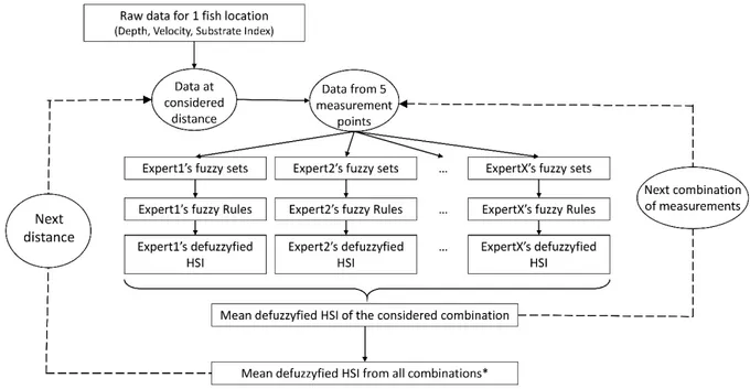
Figure 2: conceptual scheme of our study of impacts of increasing measurements distances on multiple-expert fuzzy models. (* except d310, half of combinations were performed)
164
The habitat quality was also assessed within an increasing area around the fish. The unique 165
measure realized at the exact location of the fish provided the focal data, using a mean substrate 166
size according to the proportion of different size classes, the velocity measured at 60% of the 167
depth and the depth measured using a ruler with a 1cm precision. The integration of measures 168
realized at three distances (i.e. 10, 25 and 50 cm) around the fish provided the data for the areas 169
data from the grid when they were located in the appropriate area. Then, for each distance and 172
for each fish, mean HSI was calculated from the fuzzy sets and rules developed by each expert, 173
for all of the combination of 5 measurements encompassed in the considered area (Fig. 2). The 174
mean depth, velocity and substrate size of all considered measurements were used as input data 175
in the fuzzy system. For the distance of 310 cm, half of the possible combinations of a set of 5 176
out of 16 measurements, randomly drawn, were used because of computational limitations, but 177
representing a final 50 344 combinations, and 1,066,880 HSI values. The accuracy of each model 178
was estimated with the kappa statistics (see for example McHugh, 2012), with a threshold of HSI 179
at 0.5 beyond which the habitat is considered suitable. Since presenting the HSI values did not 180
allow to visualize the variation of the HSI value for a same fish, the variation of value from the 181
HSI value at the focal point, and the mean HSI value for the considered distance were calculated 182
for each fish. The HSI values according to the distance, and then the variation with the focal HSI 183
values were compared with a Friedman two-way analysis of variance, the non-parametric test 184
corresponding to a repeat-measure ANOVA, with a post hoc analysis i.e. a Wilcoxon matched-185
pairs test with correction for multiplicity. 186
Finally, to evaluate the optimal number of environmental measurements, all measurements 187
included in a radius of 25 cm were considered for each parr (i.e. 11 measures for most of them). 188
All possible combinations of measures, including 1 to 11 measures, were averaged and a HSI 189
value was calculated for each expert fuzzy system and each fish. The accuracy of each model 190
was also estimated with the kappa statistics with a threshold of HSI at 0.5. The variation with 191
the HSI at the focal position of the fish were calculated for each expert, and then averaged for 192
each fish. The HSI variations were compared with a Friedman two-way analysis of variance with 193
a post hoc analysis (Wilcoxon matched-pairs test with correction for multiplicity). The optimal 194
number of measurements to characterize the salmon habitat was seen as the category providing 195
the highest HSI associated with fish presence and/or the smallest variability. 196
3 R E SUL T S 197
On the 10 considered sites, a total of 1366 points were sampled, showing an overall HSI mean of 198
0.42 +/- 0.12 (range from 0.17 to 0.7) for the velocity measured at 60% of the depth, and an 199
overall HSI mean of 0.48 +/-0.15 (range from 0.17 to 0.71) when velocity is measured at the 200
bottom (Tab. 1, Fig.3). 201
Table 1: Mean, minimum and maximum of Habitat Suitability Index (HSI) values from multiple-experts fuzzy system, with velocity measured at 60% of the depth (V60) and at the bottom (Vbottom), and the calculated variation at a same point, considering the entire reach of the station.
River Site Year
HSI V60 HSI Vbottom Variation
Mean Min Max Mean Min Max Mean Min Max
Catamaran Div2 2012 0.35 0.17 0.59 0.37 0.17 0.66 -0.03 -0.27 0.05 Catamaran Lor 2012 0.35 0.17 0.64 0.36 0.17 0.63 -0.01 -0.12 0.15 Catamaran Moc 2012 0.38 0.18 0.66 0.42 0.18 0.67 -0.04 -0.25 0.16 Catamaran Tom 2012 0.33 0.17 0.59 0.34 0.17 0.57 -0.01 -0.19 0.21 St-Marguerite Smp 2012-06 0.51 0.29 0.69 0.59 0.31 0.71 -0.08 -0.29 0.15 St-Marguerite Smp 2012-09 0.51 0.29 0.67 0.58 0.27 0.71 -0.07 -0.30 0.23 St-Marguerite Smt 2012-06 0.39 0.19 0.70 0.48 0.19 0.68 -0.09 -0.25 0.13 St-Marguerite Smt 2012-09 0.38 0.21 0.66 0.43 0.21 0.68 -0.05 -0.28 0.22 Miramichi Alx 2012 0.53 0.30 0.69 0.65 0.30 0.71 -0.12 -0.31 0.03
202
Figure 3: Map of HSI value distribution, after spline interpolation from measuring points (white stars), for velocity measured at the bottom (left panel) or at 60% of the depth in the water column (middle panel), and the difference between them (right panel), in the Miramichi River (Spm site).
The two sets of HSI were significantly different (Wilcoxon matched-pairs signed-ranks test with 203
correction for multiplicity, pvalue < 2.2e16). The variations of HSI values were ranged from -204
0.30 to +0.23 (mean= -0.06 +/-0.09). 205
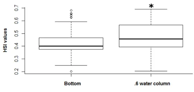
In the three rivers, 93 fish were observed. HSI were calculated at the focal location of the fish, 206
using the velocity measured at the bottom, then at 60% of depth (Fig.4). The resulting HSI 207
values were significantly higher (Wilcoxon matched-pairs signed-ranks test, p-value <0.001), 208
when the velocity was measured at 60% of the depth (mean= 0.47 +/- 0.11) than at the bottom 209
(mean= 0.42 +/- 0.1). 210
Figure 4: Distribution of HSI values with velocity measured at the bottom (left panel) or at 60% of the depth (right panel) at the exact fish location. Asterisks (*) indicate significant difference (Wilcoxon matched-pairs signed-ranks test, p-value <0.001).
211
Regarding the influence of increasing area of measures around the fish, 7 distances were tested: 0 212
(focal measure), 10, 25, 50, 113, 190 and 310 cm around the parr (Tab.2, Fig.5). The focal 213
measures provided the lowest mean HSI and the largest variability (mean= 0.47 +/- 0.11). The 214
HSI increased slowly until d50, and decreased afterward, while the variability decreased 215
progressively. Regarding the variation of HSI by fish, the highest positive difference with the 216
focal HSI value occurred at d50 (mean= +3.92.10-2 +/- 6.35.10-2) and the highest kappa value is 217
reached at the same distance (κ = 0.66 at d50; Tab.2). Friedman’s test was significant for the HSI 218
other significant difference was found afterwards. The same analysis on the variation with the 221
focal values highlighted significant differences between every distances (all p-value <0.05) but 222
d113 and d190 (p-value= 0.28). 223
Table 2: mean values and standard deviation (SD) for HSI values, and for the variation from the focal HSI values for each parr, provided by a multiple-expert fuzzy system on every possible combination of 5 measures encompassed in seven increasing distances
(0, 10, 25, 50, 113, 190 and 310 cm) around the considered parr.
Distance Mean HSI SD HSI
Mean variation with focal values
SD variation with focal values d0 0.475 0.112 0 0 d10 0.499 0.106 0.024 0.058 d25 0.506 0.105 0.031 0.062 d50 0.514 0.099 0.039 0.064 d113 0.514 0.095 0.039 0.07 d190 0.514 0.096 0.039 0.08 d310 0.512 0.096 0.037 0.082 224 225
Figure 5: Distribution of HSI values calculated with a multiple-experts fuzzy model (left panel) and the variation of this HSI values with the focal HSI value for each parr (right panel), according to the distance inside which measures were considered as input data for the model; the HSI values (lines) of a selection of 6 (out of 93) different fish are provided. Asterisks (*) indicate a significant difference with the other categories. Daggers (†) indicate non-significant difference between the two categories, all other differences are significant (both post hoc Wilcoxon matched-pairs signed-ranks test).
226
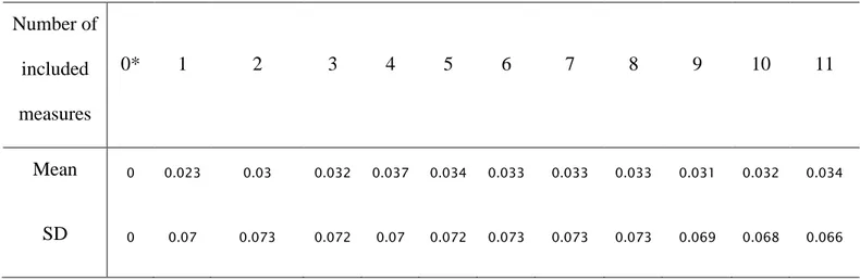
For the number of measurements to include in the models, the HSI provided by the different 227
categories of included measures were averaged for each fish and for each expert. All HSI 228
calculated showed an increase compared with the value calculated from the focal position 0*. 229
The maximum is reached with 11 measures but the Cohen’s kappa was the highest with 6 230
measures (κ = 0.66), providing 94% of the maximum improvement of HSI values (Tab. 3, Fig. 231
6). The variations of HSI values between categories were significantly different from each other 232
significant differences with each other (Wilcoxon matched-pairs signed-ranks test, p-value <0.01 234
for these three categories, p-value >=0.42 for the other combinations). 235
Table 3: Means and standard deviations of differences in values of calculated HIS, between focal environmental measures of Salmon parr location (0*) and averaged HSI from every combination of
measures, including from 1 to 11 measures.
Number of included measures 0* 1 2 3 4 5 6 7 8 9 10 11 Mean 0 0.023 0.03 0.032 0.037 0.034 0.033 0.033 0.033 0.031 0.032 0.034 SD 0 0.07 0.073 0.072 0.07 0.072 0.073 0.073 0.073 0.069 0.068 0.066 236
Figure 6: Differences in values of calculated HSI, between focal environmental measures of salmon parr location (0*) and averaged HSI from every combination of measures, including 1 to 11 measures; the differences in HSI values (lines) of a selection of 7 (out of 93) different fish are provided. Asterisks (*) indicate categories with no significant differences from each other (post hoc Wilcoxon matched-pairs signed-ranks test).
237
4 DI SC USSI ON 238
Highlighting and calculating the radial distance from the fish defining a circle in which 239
were tested for each presence. The null distance, i.e. the focal measure taken at the exact location 242
of the fish, gave globally the lowest HSI values and the highest variability. This is potentially 243
explained by the fact that only one measurement of each habitat variable may introduce an 244
important bias: assuming the fact that the parr may chose a suboptimal focal location with good 245
vicinity, if the exact location did not present good conditions for the fish, the error is not 246
attenuated by other measurements. Consequently, despite the geographic proximity of their 247
measures, the multiple-measures 10 cm-distance and the unique focal measure showed 248
significant differences in their calculated HSI, the 10 cm-distance providing a slightly better HSI 249
than focal measurements. Then, increasing the distance improved the model performance: for a 250
same fish, the HSI calculated by the fuzzy system reached a peak at a distance of 50 cm, which 251
corresponded with an area of 0.79 m², consistent with previous assessment of parr territory sizes 252
(Keeley & Grant, 1995; Lindeman et al., 2015). Beyond this distance, the calculated HSI values 253
tend to remain constant, the loss of variability in HSI values being the sign of a homogenization 254
of the measures at a large scale instead of a model improvement, as proved by the large 255
variability of HSI values at large distance. 256
Our protocol gave the opportunity to explore the influence of the location of the velocity 257
measurements in an expert fuzzy system. As expected, the data highlighted the fact that the 258
velocities at the bottom were slower than at 60%, because of frictions with the substrate, and 259
sometimes even counter-currents were observed. Near the bottom, parr can save some energy 260
while having access to the drifting food, the habitat quality should be consequently higher there 261
than further up in the water column. The HSI values were slightly lower when the velocities 262
were measured at the bottom than at 60% of total depth. In addition, with the measurements 263
taken at the fish location, our result showed an improvement of the model with higher HSI when 264
depth instead of at the bottom for a benthic fish is unexpected and raises some questions. It is 266
unclear if the experts unconsciously referred to the velocity in the middle of the water column 267
when they built their memberships functions and rules, or if they consider the 60%-depth 268
velocity is more representative of the velocity associated with the drifting food. 269
It is usual, when characterizing salmon habitat, to take one measure of velocity and depth, and 270
an assessment of the substrate at the exact location of the fish. Our results showed that the values 271
of HSI provided by one measure at the exact location of the fish were generally lower than 272
several measures realized in its direct environment. The average highest HSI value was obtained 273
when all the measurements of each habitat variable, at randomly selected locations (within a 274
radius of 25 cm), were aggregated, but 6 measurements provided the best model. More than 6 275
measurements improved marginally the model outputs and the extra time and efforts required is 276
not warranted in this case. However, a fixed number of measurements to describe the 277
environmental conditions cannot be applicable to every circumstance and should be adapted to 278
local habitat complexity. In addition, our results exhibit a snapshot of habitat suitability, for a 279
short time period and the integration of flow dynamics would be important to model adequately 280
the salmon habitat (Boavida, Harby, Clarke, & Heggenes, 2017). Nevertheless, our study shows 281
a clear difference in the models outputs, highlighting the needs to take into consideration 282
multiple measurements in a close range around the individuals. 283
Our results suggest that the best description of the parr rearing habitat during summer diurnal 284
period to be used in the fuzzy logic model described by Mocq et al. (2013) is reached by taking 285
into consideration the neighboring conditions, i.e. measuring variables at 50 cm from the fish and 286
adding them to calculate a mean value. In addition, this multiple-points sampling protocol could 287
part of its territory instead of only its home-rock, as our results indicate. Our hypothesis about 290
the model efficiency was that a high calculated HSI for a presence indicated that habitat 291
description used in the calculations was accurate and consequently, led to a more efficient model. 292
However, parr were frequently present in habitats with calculated HSI under 0.5, while the 293
reaches presented large bands of good quality. Field observations indicate that, in the three 294
sampled rivers, densities extended from 0.5 to 13.5 ind/100 m², were too low to force some parr 295
to use poor-quality habitat. Therefore, density dependence-related biases are not the likely cause 296
of presence of fish in relatively poor habitat. This observation can more likely be explained by 297
expert’s unsure or ill-translated knowledge in the fuzzy sets and rules. These biases are found in 298
the fuzzy sets and rules definition: the unsure or ill-defined knowledge could be represented in 299
fuzzy logic by an important overlap between successive categories or by membership functions 300
limits irrelevant with ecological reality. Indeed, accurate codification of the expert knowledge is 301
an important obstacle. The difficulties could come from the expert (unwanted forgetting of 302
information, difficulty of expression or abstraction, fear of personal knowledge disclosure and 303
use; Chevrie and Guély, 1998, Drescher et al., 2013), or from the method (poor ergonomics of 304
the worksheet used to collect data, lack of precision in words or concepts description; Knol et al., 305
2010). In addition, the growth of the parr evolves quickly in few months, especially for the 306
youngest parr, modifying their habitat preferences and complicating the definition of the related 307
fuzzy sets. Finally, another explanation could be related with the physical factors that were not 308
included in the model: indeed, the habitat selection by parr is under the influences of multiple 309
factors (Armstrong et al., 2003), generally of lesser importance than the three selected variables 310
but sufficiently important to modify substantially the habitat selection of some of the fish. 311
This study is linked to the problematic study of scale, i.e. the spatial and temporal dimension of 312
physical habitat, some studies work at the microhabitat scale, measuring environmental physical 314
variables in the vicinity of the fish, on the order of the cm² (Armstrong et al., 2003; Heggenes et 315
al., 1995; Heggenes, Bagliniere, & Cunjak, 1999). By contrast, other studies are concerned with 316
the mesohabitat scale, from m² to some tens of m², equivalent to Channel Morphological Units 317
(CMU, e.g. riffle, glide, pool; Folt et al., 1998). For the habitat characterization, the mesohabitat 318
is too large to precisely describe salmon needs and preferences, while the microhabitat neglects 319
environmental elements which could influence the selection and the occupation of the habitat by 320
the fish (Shirvell, 1994). An intermediate scale, considering the exact location of the fish and its 321
close environment as potential used habitat, could be useful to describe more precisely the 322
habitat and improve the model predictions. Moreover, lots of scientific studies and protocols 323
about fish habitat are based, for their field data, on the measures of environmental variables at 324
the exact location of the fish: our results suggest a change in this protocol may be needed, in 325
order to improve the habitat description. 326
Acknowledgements 327
The authors wish to acknowledge every expert who agreed to participate in this study: 328
Alfredsen K., Belles-Isles M., Belzile L., Bergeron N., Bérubé M., Boivin A., Breau C., Buoro 329
M., Caron F., Clément M., Cuerrier D., Cunjak R., Dauphin G., Dumont R., Gauthier C., 330
Guérard N., Heggenes J., Johnston P., Lapointe A., Lesvesque F., Linnansaari T., Milner N., 331
Moore D., Murdock M., Noak M., Prevost E., Riley B., Rodriguez M., Sabourin F., Saltveit S.J. 332
and their respective organizations. We thank Genivar Consulting for hydraulic model outputs, 333
and A. Maheu, A. Blanchette, M. Samsom-Do and the crew of the UNB for their help on field. 334
Funding: This work was supported in part by NSERC, Hydro-Québec and the Institut National 336
de la Recherche Scientifique (INRS). 337
R eferences 338
Armstrong, J. D., Kemp, P. S., Kennedy, G. J. A., Ladle, M., & Milner, N. J. (2003). Habitat 339
requirements of Atlantic salmon and brown trout in rivers and streams. Fisheries Research, 340
62(2), 143–170. http://doi.org/Pii S0165-7836(02)00160-1 341
Bardonnet, A., & Baglinière, J.-L. (2000). Freshwater habitat of Atlantic salmon (Salmo salar). 342
Canadian Journal of Fisheries and Aquatic Sciences, 57(2), 497–506. 343
Benyahya, L., Daigle, A., Caissie, D., Beveridge, D., & St-Hilaire, A. (2009). Caractérisation du 344
régime naturel du débit des bassins versants de l’Est du Canada (Vol. Rapport R1). INRS-345
ETE. 346
Boavida, I., Harby, A., Clarke, K. D., & Heggenes, J. (2017). Move or stay: habitat use and 347
movements by Atlantic salmon parr (Salmo salar) during induced rapid flow variations. 348
Hydrobiologia, 785(1), 261–275. http://doi.org/10.1007/s10750-016-2931-3 349
Chevrie, F., & Guély, F. (1998). Cahier technique n°191: La logique floue. Groupe Schneider. 350
Cunjak, R., Caissie, D., & El-Jabi, N. (1990). The Catamaran Brook Habitat Research Project: 351
Description and General Design of Study. Canadian Technical Report of Fisheries and 352
Aquatic Sciences (Vol. 1751). Moncton: Department of Fisheries and Oceans. 353
Cunjak, R., Caissie, D., el-Jabi, N., Hardie, P., Conlon, J. H., Pollock, T. L., … Komadina-354
Douthwright, S. (1993). The Catamaran Brook (New Brunswick) Habitat Research Project: 355
Biological, Physical and Chemical Conditions (1990-1992). Canadian Technical Report 356
of Fisheries and Aquatic Sciences. Moncton: Department of Fisheries and Oceans. 357
Drescher, M., Perera, A. H., Johnson, C. J., Buse, L. J., Drew, C. A., & Burgman, M. A. (2013). 358
Toward rigorous use of expert knowledge in ecological research. Ecosphere, 4(7), 1–26. 359
http://doi.org/10.1890/ES12-00415.1 360
15(3), 579–590. http://doi.org/10.1577/1548-8675(1995)015<0579:TUOWDA>2.3.CO;2 363
Foldvik, A., Einum, S., & Finstad, A. G. (2016). Spatial diffusion modelling of juvenile Atlantic 364
salmon (Salmo salar) shows ontogenetic increase in movement rates. Canadian Journal of 365
Fisheries and Aquatic Sciences, 1–6. http://doi.org/10.1139/cjfas-2015-0315 366
Folt, C. L., Nislow, K. H., & Power, M. E. (1998). Implications of temporal and spatial scale for 367
Atlantic salmon (Salmo salar) research. Canadian Journal of Fisheries and Aquatic 368
Sciences, 55, 9–21. 369
Fukuda, S., & Hiramatsu, K. (2008). Prediction ability and sensitivity of artificial intelligence-370
based habitat preference models for predicting spatial distribution of Japanese medaka 371
(Oryzias latipes). Ecological Modelling, 215(4), 301–313. Retrieved from 372
http://www.sciencedirect.com/science/article/B6VBS-4SK2V3R-373
1/2/49220e5317c43e908ca2066127001686 374
Gerking, S. D. (1953). Evidence for the Concepts of Home Range and Territory in Stream 375
Fishes. Ecology, 34(2), 347–365. Retrieved from http://www.jstor.org/stable/1930901 376
Grant, J. W. A., Steingrimsson, S. O., Keeley, E. R., & Cunjak, R. A. (1998). Implications of 377
territory size for the measurement and prediction of salmonid abundance in streams. 378
Canadian Journal of Fisheries and Aquatic Sciences, 55, 181–190. 379
Guay, J. C., Boisclair, D., Rioux, M., Leclerc, M., Lapointe, M., & Legendre, P. (2000). 380
Development and validation of numerical habitat models for juveniles of Atlantic salmon 381
(Salmo salar) (Vol. 57). Ottawa, ON, CANADA: National Research Council of Canada. 382
Hedger, R. D., Dodson, J. J., Bergeron, N. E., & Caron, F. (2005). Habitat selection by juvenile 383
Atlantic salmon: the interaction between physical habitat and abundance. Journal of Fish 384
Biology, 67(4), 1054–1071. http://doi.org/10.1111/j.0022-1112.2005.00808.x 385
Heggenes, J. (1990). Habitat utilization and preferences in juvenile atlantic salmon (salmo salar) 386
in streams. Regulated Rivers: Research & Management, 5(4), 341–354. 387
http://doi.org/10.1002/rrr.3450050406 388
Heggenes, J., Bagliniere, J. L., & Cunjak, R. (1995). Note de synthèse sur la sélection de niche 389
Pisciculture, (337-338–339), 231–239. Retrieved from 392
http://dx.doi.org/10.1051/kmae:1995026 393
Heggenes, J., Bagliniere, J. L., & Cunjak, R. A. (1999). Spatial niche variability for young 394
Atlantic salmon (Salmo salar) and brown trout (S-trutta) in heterogeneous streams. Ecology 395
of Freshwater Fish, 8(1), 1–21. 396
Heland, M., & Dumas, J. (1994). Ecologie et comportements des juvéniles. In J. Guéguen & P. 397
Prouzet (Eds.), Le Saumon Atlantique (pp. 29–46). Ifremer. 398
Höjesjö, J., Kaspersson, R., & Armstrong, J. D. (2015). Size-related habitat use in juvenile 399
Atlantic salmon: the importance of intercohort competition. Canadian Journal of Fisheries 400
and Aquatic Sciences, 73(8), 1182–1189. http://doi.org/10.1139/cjfas-2015-0446 401
Johnston, T. A. (1997). Downstream movements of young-of-the-year fishes in Catamaran 402
Brook and the Little Southwest Miramichi River, New Brunswick. Journal of Fish Biology, 403
51(5), 1047–1062. http://doi.org/10.1111/j.1095-8649.1997.tb01543.x 404
Jorde, K., Schneider, M., Peter, A., & Zoellner, F. (2001). Fuzzy based models for the evaluation 405
of fish habitat quailty and instream flow assessment. Proceedings of the 3rd International 406
Symposium on Environmental Hydraulics. Tempe, AZ. 407
Keeley, E. R., & Grant, J. W. A. (1995). Allometric and environmental correlates of territory size 408
in juvenile Atlantic salmon (Salmo salar). Canadian Journal of Fisheries and Aquatic 409
Sciences, 52(1), 186–196. http://doi.org/10.1139/f95-019 410
Knol, A., Slottje, P., van der Sluijs, J., & Lebret, E. (2010). The use of expert elicitation in 411
environmental health impact assessment: a seven step procedure. Environmental Health, 412
9(1), 19. Retrieved from http://www.ehjournal.net/content/9/1/19 413
Lewis, C. A., Lester, N. P., Bradshaw, A. D., Fitzgibbon, J. E., Fuller, K., Hakanson, L., & 414
Richards, C. (1996). Considerations of scale in habitat conservation and restoration. 415
Canadian Journal of Fisheries and Aquatic Sciences, 53(S1), 440–445. 416
http://doi.org/10.1139/f96-021 417
Lindeman, A. A., Grant, J. W. A., & Desjardins, C. M. (2015). Density-dependent territory size 418
and individual growth rate in juvenile Atlantic salmon (Salmo salar). Ecology of Freshwater 419
Mäki-Petäys, A., Erkinaro, J., Niemelä, E., Huusko, A., & Muotka, T. (2004). Spatial 421
distribution of juvenile Atlantic salmon (Salmo salar) in a subarctic river: size-specific 422
changes in a strongly seasonal environment. Canadian Journal of Fisheries and Aquatic 423
Sciences, 61(12), 2329–2338. http://doi.org/10.1139/f04-218 424
Mamdani, E. H. (1977). Application of fuzzy logic to approximate reasoning using linguistic 425
synthesis. Proceedings of the Sixth International Symposium on Multiple-Valued Logic. 426
Logan, Utah, United States: IEEE Computer Society Press. 427
McHugh, M. L. (2012). Interrater reliability: the kappa statistic. Biochemia Medica, 22(3), 276– 428
282. Retrieved from http://www.ncbi.nlm.nih.gov/pmc/articles/PMC3900052/ 429
Mocq, J., St-Hilaire, A., & Cunjak, R. a. (2015). Influences of Experts’ Personal Experiences in 430
Fuzzy Logic Modeling of Atlantic Salmon Habitat. North American Journal of Fisheries 431
Management, 35(2), 271–280. Retrieved from
432
http://www.tandfonline.com/doi/full/10.1080/02755947.2014.996684 433
Mocq, J., St-Hilaire, A., & Cunjak, R. A. (2013). Assessment of Atlantic salmon (Salmo salar) 434
habitat quality and its uncertainty using a multiple-expert fuzzy model applied to the 435
Romaine River (Canada). Ecological Modelling, 265, 14–25. 436
Morantz, D. L., Sweeney, R. K., Shirvell, C. S., & Longard, D. A. (1987). Selection of 437
Microhabitat in Summer by Juvenile Atlantic Salmon (Salmo salar). Canadian Journal of 438
Fisheries and Aquatic Sciences, 44(1), 120–129. http://doi.org/10.1139/f87-015 439
Mouton, A. M., Schneider, M., Peter, A., Holzer, G., Müller, R., Goethals, P. L. M., & De Pauw, 440
N. (2008). Optimisation of a fuzzy physical habitat model for spawning European grayling 441
(Thymallus thymallus L.) in the Aare river (Thun, Switzerland). Ecological Modelling, 442
215(1–3), 122–132. http://doi.org/10.1016/j.ecolmodel.2008.02.028 443
Muñoz-Mas, R., Papadaki, C., Martínez-Capel, F., Zogaris, S., Ntoanidis, L., & Dimitriou, E. 444
(2016). Generalized additive and fuzzy models in environmental flow assessment: A 445
comparison employing the West Balkan trout (Salmo farioides; Karaman, 1938). Ecological 446
Engineering, 91, 365–377. http://doi.org/http://dx.doi.org/10.1016/j.ecoleng.2016.03.009 447
Rykiel, E. J. (1996). Testing ecological models: the meaning of validation. Ecological 451
Modelling, 90(3), 229–244. http://doi.org/10.1016/0304-3800(95)00152-2 452
Schoeneberger, P. J., Wysocki, D. A., Benham, E. C., Soil Survey Staff, & Natural Resources 453
Conservation Service, N. S. S. C. (2012). Field Book for Describing and Sampling Soils, 454
version 3.0. Lincoln, NE: Natural Resources Conservation Service, National Soil Survey 455
Center. 456
Shepard, R. B. (2005). Quantifying Environmental Impact Assessment Using Fuzzy Logic. (B. N. 457
Anderson, R. W. Howarth, & L. R. Walker, Eds.). New-York: Springer. 458
Shirvell, C. S. (1994). Effect of changes in streamflow on the microhabitat use and movements 459
of sympatric juvenile coho salmon (Oncorhynchus kisutch) and chinook salmon (O. 460
tshawytscha) in a natural stream. Can. J. Fish. Aquat. Sci., 51(7), 1644–1652. 461
Wildman, T. L., & Neumann, R. M. (2003). Comparison of snorkeling and electrofishing for 462
estimating abundance and size structure of brook trout and brown trout in two southern New 463
England streams. Fisheries Research, 60(1), 131–139. http://doi.org/10.1016/s0165-464
7836(02)00060-7 465