This is an accepted manuscript of an article published by Elsevier in Landscape and Urban Planning in January 2017, available at http://dx.doi.org/10.1016/j.landurbplan.2016.09.001 This manuscript version is made available under de CC-BY-NC-ND 4.0 license
http://creativecommons.org/licenses/by-nc-nd/4.0/ Please cite as:
Pham, Thi-Thanh-Hien, Philippe Apparicio, Shawn Landry, and Joseph Lewnard. 2017.
"Disentangling the effects of urban form and socio-demographic context on street
tree cover: A multi-level analysis from Montréal." Landscape and Urban Planning
157:422-433. doi: 10.1016/j.landurbplan.2016.09.001.
Abstract
1
Street trees provide a wide range of benefits for cities. Street tree cover (STC) is explained by
2
urban form, social stratification and lifestyle theories that operate at multiple scales. In this paper
3
we examine how the urban form (street characteristics), social stratification and lifestyle
(socio-4
demographics) account for variations of STC in Montréal. Tree cover was identified from Quickbird
5
images and then overlaid on street segments to compute the STC. Each street segment was nested
6
in a census tract. We used 2-level models with mixed effects and interactions (between street
7
attributes and demographic variables) while introducing a spatial term. Political,
socio-8
economic or other explanatory factors operating at the tract level can potentially explain 17.6% of
9
the variation of STC. Overall, the street characteristics explained more variation in STC than the
10
socio-demographic context. Lifestyle is less important than social stratification. Street length is
11
positively associated with STC; street width and the percentage of duplexes and triplexes are
12
negatively associated with STC, while construction age has a u-shaped effect on STC. Interactions
13
show that STC is higher in expensive and highly-educated areas that have residential streets or
14
streets with large setback (sidewalk). Areas predominantly comprised of low-income households
15
could have higher or lower STC depending on the number of buildings and the percentage of
16
duplexes and triplexes. Streetscape and socio-demographic contexts intertwine to create complex
17
patterns of STC. Greening programs should be designed carefully according to local contexts since
18
certain types of greening can lead to gentrification and displacement of low-income households.
19
INTRODUCTION
21
Trees in cities provide a wide range of benefits for urban dwellers. Trees and tree canopy provide
22
ecosystem services such as urban heat mitigation, stormwater runoff reduction and filtering, and
23
noise reduction (see Mullaney et al. (2015) and Roy et al. (2012)). The presence of trees or tree
24
canopy in neighborhoods has been correlated with the following benefits for inhabitants:
25
increased physical activity (Sarkar et al., 2015), improved mental health (Taylor et al., 2015),
26
improved physical health (through stress reduction and increased social cohesion) (de Vries et al.,
27
2013), and less crime (Donovan & Prestemon, 2012; Troy et al., 2012). Street trees are also highly
28
associated with street walkability and livability (Sarkar et al., 2015).
29
At the same time, urban trees are sources of nuisances or disservices, as termed by some authors
30
(Lyytimäki & Sipilä, 2009). For example, a review by Lyytimäki and Sipilä (2009) shows urban trees
31
may cause damage to physical structures (tree roots, which break up pavements, or tall trees,
32
which may cause maintenance problems), compromise security (green areas are sometimes
33
perceived as unsafe by women) and give rise to health issues (allergies, poisoning). People’s
34
perceptions of what they consider to be services and disservices of urban green areas vary across
35
ethno-cultural and demographic groups (Lyytimäki & Sipilä, 2009). Research on the disservices of
36
urban trees that merits increased attention from scholars and public agencies in order to better
37
maximize services and minimize disservices.
38
Despite such nuisances, studies across various urban contexts increasingly show that urban
39
dwellers from different socio-economic groups highly value and recognize the benefits from trees
40
(Mullaney et al., 2015; Peckham et al., 2013; Shackleton et al., 2015). In the context of rising
41
concerns about urban heat islands and increased flooding due to climate change, investing in
42
green infrastructure in general and trees in particular is politically and socially appealing for urban
43
planners and administrators (Matthews et al., 2015). Cities all over the world are promoting trees
44
in general and street trees specifically (Silvera Seamans, 2013) as a means to improve
45
sustainability.
46
However, evidence from many cities is showing that urban vegetation in general and street trees
47
in particular are not equally distributed according to socio-economic status. More specifically,
48
across North American cities, low-income households and certain ethno-cultural groups of the
49
population tend to have limited access to trees as well as to benefits provided by trees (e.g. Landry
50
& Chakraborty, 2009; Pham et al., 2012; Schwarz et al., 2015; Tooke et al., 2010). Furthermore,
51
urban greening can result in paradoxical effects, such as increased housing values, gentrification
52
and displacement of low-income people (Wolch et al., 2014). Greening can also lead to negative
53
and unexpected reactions from the public, as the public may not understand benefits provided by
54
street trees. For example in New York City citizen complaints about the ‘New Street Tree’ program
55
were mostly found in areas that had new plantings (Rae et al., 2010).
56
The uneven distribution of urban trees and the complexity of ensuring environmental equity raise
57
questions about the physical, ecological and socio-economic correlates as well as the underlying
58
mechanisms associated with urban tree distributions. The distribution of street trees can be
city-59
specific since public policies concerning this issue are determined on the basis of site-specific
60
factors such as climate, geographic conditions, history and preferences (Kirkpatrick et al., 2011).
61
While there is a growing body of literature addressing urban tree cover at the household or parcel
62
scale of analysis, many of these studies focus on residential tree cover rather than on street trees
63
or street tree cover (e.g. Chowdhury et al., 2011; Larson et al., 2010; Shakeel & Conway, 2014). In
64
this article, we focus on street trees. We use street tree cover, hereinafter referred to as “STC”, as
65
an indicator of the presence of street trees.
66
Studies addressing correlates of street trees focus mostly on socio-economic factors that have
67
been reported at larger geographic scales, such as suburbs in Australia, census block groups in the
68
United States or dissemination areas in Canada (Kirkpatrick et al., 2011; Landry & Chakraborty,
69
2009; Pham et al., 2013), with only one study (from Bangalore, India) looking at street
70
characteristics (Nagendra & Gopal, 2010). The three Western studies were conducted in very
71
different cities in terms of climate conditions and population density and with different sets of
72
correlates. Kirkpatrick et al. (2011) used two income variables in suburbs of six Australian cities.
73
Landry et al. (2009), examining street trees from an equity angle, used socio-demographic
74
variables and one variable related to the built environment (median housing age) in Tampa,
75
Florida (United States). Pham et al. (2013) looked at socio-demographic variables and two proxies
76
of the built environment (population density and construction age of parcels) in Montréal, Canada.
77
The study conducted in India by Nagendra and Gopal (2010) examined the distribution and
78
diversity of street trees in relation to street width. To our knowledge there is no study that has
79
examined the role of the physical characteristics of streets in shaping STC in an exhaustive way.
80
More importantly, a large geographic unit (e.g., a block group) typically contains multiple street
81
segments, whereby the coarser resolution of the analysis may mask the heterogeneity of physical
82
characteristics of streets that could be associated with the distribution of STC, e.g., age of housing
83
construction, building density, housing types, presence of a sidewalk and land use. The dispersed
84
scholarship on street trees shows important differences among the studied cities, sometimes
85
presenting contradictory evidence and with few studies presenting an analysis at fine spatial
86
resolutions. For example, Nagendra and Gopal (2010) in their study on Bangalore found that
87
narrow roads had fewer trees and smaller sized trees while wide streets had large trees. The fact
88
that narrow streets, more likely to be residential, have fewer trees or lower tree cover suggests
89
that big trees are not found in areas where the population’s need for ecosystem services is
90
highest. Yet Kirkpatrick et al. (2011) witnessed that there was no difference between wide and
91
narrow streets in Hobart (Australia). This wide range of findings makes it difficult to theorize about
92
mechanisms underlying STC and to make generalizations about environmental inequities in tree
93
benefits that could inform urban planning priorities.
94
Drawing on urban form, social stratification and lifestyle theories that explain urban vegetation
95
(Bigsby et al., 2013; Lowry et al., 2012; Sanders, 1984) our paper investigates correlates of STC at
96
the fine scale of the street level while also considering the socio-economic context of the
97
neighborhood in the case of Montréal (Canada). We use a multi-level and mixed modeling
98
approach to capture the effects of these theories simultaneously at the street and neighborhood
99
scales. We ask the following research questions: 1) To what extent do street-level physical
100
attributes and socio-demographic factors of context account for variation in STC? 2) Which set of
101
correlates is more important? 3) How do street attributes interact with socio-economic context
102
when shaping STC? By exploring these questions, we hope to enrich the discourse about urban
103
tree cover and raise awareness of the topic of street trees in general.
104
THE CASE OF MONTRÉAL
105
This study is conducted on the territory of the City of Montréal before the municipal reform in
106
2002. The city was composed of nine boroughs, a political jurisdiction of Montréal, covering 149
107
km2 (Fig 1). In 2006, that area had a population of more than one million people and a population
108
density ranging from 12,000 inhabitants/km2 in the central boroughs to 5,000 people/km2 on the
109
outskirts. Of the residential dwellings, 64% were apartments in buildings with fewer than five
110
stories; 14% were apartments in duplexes (two dwellings located one above the other in the
111
building); 10% were single- and semi-detached houses; and 8% were apartments in high-rise
112
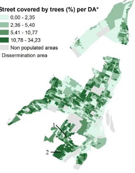
buildings (Statistics Canada, 2006). The percentage of streets covered by trees is mapped in Figure
113
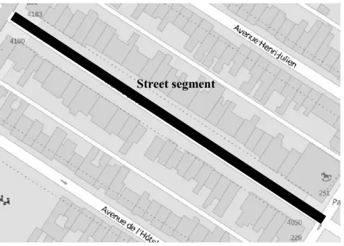
2.
114
Figure 1. Location and population density of the former City of Montréal, by dissemination area
115
(Statistics Canada, 2006)
116
117
Figure 2. Percentage of streets covered by trees, in the former City of Montréal (aggregated by
118
dissemination area)
119
120
Due to an invasion of the Emerald Ash Borer (Agrilus planipennis) starting in 2011, the City began
121
cutting down 10,000 ash trees on its streets, being the equivalent of 20% of the ash tree
122
population. To compensate for this loss and to address other goals such as mitigating the urban
123
heat island effect, the City is now aiming to increase its citywide tree canopy coverage from 20%
124
to 25% by 2021. For this it plans to plant 300,000 trees, of which 75,000 are street trees and other
125
public trees, together costing over $68 million Canadian dollars (City of Montréal, 2011). Here, a
126
greater knowledge and understanding of the physical and socio-economic factors that influence
127
STC at the scale of the street level could serve Montréal and other cities to efficiently maintain and
128
expand an equitable and sustainable STC (City of Montréal, 2011) and to identify the areas that
129
are deprived in terms of street trees.
130
THEORIZING AND MODELLING STREET TREE COVER
131
As proposed by Sanders (1984) and then developed by other authors (e.g. Berland et al., 2015;
132
Bigsby et al., 2013; Lowry et al., 2012; Troy et al., 2007), the distribution of the urban forest is
133
generally affected by three groups of factors: natural factors (e.g., climate, underlying biome, soils,
134
elevation, slope), the urban form (e.g., population density and urban morphology) and drivers of
135
vegetation management systems (e.g., residential landscaping decisions or public management
136
related to social stratification, lifestyle/ecology of prestige, luxury effects). Some authors have
137
recently shown that in specific geographical conditions natural factors are dominant in shaping
138
urban tree cover. For example, in Cincinnati (characterized by a high variability of elevation)
139
Berland et al. (2015) found hilly areas have more trees and these areas are inhabited by either
140
white wealth people or black people. This is explained by historical segregation of the city. In Salt
141
Lake County, a semi- and arid environment, Lowry et al. (2012) found that annual precipitation
142
and aspects (westness) have significant associations with residential tree canopy. As Montreal
143
does not have very specific natural conditions, we did not consider natural factors in our study.
144
Our theoretical framework is hence designed to consider three theories that explain the
145
distribution of STC: urban form, social stratification and lifestyle.
146
Urban form
147
This theory builds on and nuances the population density theory which has been put forth to
148
explain the driver of urban vegetation (Troy et al., 2007). The population density theory posits that
149
because people displace native ecosystems, areas with higher population density have less
150
physical space available for urban vegetation. However, empirical research has shown that the
151
relationship between tree cover and population density varies in direction and magnitude from
152
one city to another. For example, the relationship was found to be negative in Baltimore (Troy et
153
al., 2007) and Denver (Mennis, 2006); positive in multiple Australian cities (Luck et al., 2009); and
154
not significant in Toronto (Conway & Hackworth, 2007). In Montréal, Pham et al. (2013) found a
155
negative relationship between residential tree cover and population density, but a positive
156
relationship between STC and population density. In their work in Raleigh and Baltimore, Bigsby et
157
al. (2013) suggest that population density was generally less important than measures of the
158
urban form such as pervious areas and parcel size. Overall, the research therefore suggests that
159
the population density theory alone is insufficient as an explanation of urban vegetation.
160
The urban form theory also states that tree cover depends largely on the space available for
161
planting. Space available for planting is determined by a set of factors such as parcel size, land use
162
patterns, age of neighborhoods, block perimeter and street density (Bigsby et al., 2013; Conway &
163
Urbani, 2007; Mennis, 2006). Lowry et al. (2012) further characterize urban sprawl using five
164
factors: street connectivity, land use mix, median lot size, residential street density and median
165
block perimeter.
166
Tree survival studies have shown that urban trees are more likely to survive in wider rather than
167
narrow tree pits (Koeser et al., 2013; Lu et al., 2010; Nowak et al., 1990). Tree pit size depends
168
mostly on the size of sidewalk and building setback (i.e., distance from road to building). Parcel or
169
neighborhood development age is widely discussed in studies of urban vegetation (Conway &
170
Urbani, 2007; Landry & Pu, 2010; Mennis, 2006). The relationship between the age of the
171
development and the vegetation has been found to be u-shape, in other words, tree cover was
172
found to peak in neighborhoods of a certain age and then decline (Grove et al., 2006; Landry & Pu,
173
2010). This relationship reflects the natural lifecycle of trees (as the neighborhood gets older, trees
174
grow to their full canopy and then die) and the changes in planning practices over time.
175
Such numerous variables characterizing the urban form need to be considered in appropriate
176
scales. In a dense city such as Montréal, having a complex urban form due to its diverse housing
177
patterns, we believe that the street level is a more appropriate scale than census block group or
178
dissemination area level to examine STC.
179
Social stratification
180
The social stratification theory can explain how residents with differential socio-economic statuses
181
can influence tree planting and management on public and private lands, or choose to locate in
182
areas with more green amenities. Two variations of this theory can be used to explain the
183
distribution of trees on public lands, including street trees. The “mobility” explanation suggests
184
that people with greater economic means will move to locations with more amenities such as
185
trees (Troy et al., 2007). The mobility explanation will not be considered in this study because it
186
requires long-term data of residential patterns and real estate markets. The second explanation,
187
proposed by Logan and Molotch (1987), is that people with differential access to power and
188
income can influence public investment in amenities such as trees (Grove et al., 2006).
189
According to this theory, tree cover is influenced by socio-economic factors at two geographic
190
levels, one being the individual/household level and the other the neighborhood level. At the
191
former level, tree cover is influenced by landscape decisions of home owners, and at the latter
192
through support for public or private management. In this paper, which focuses on public trees,
193
we examine the socio-economic factors at play at the neighborhood level, such as how citizens
194
take part in decision-making to channel municipal investment toward planting and greening
195
activities or how they promote private investments from developers, grassroots organizations or
196
NGOs to this effect (Conway et al., 2011). The following variables are usually used to represent
197
social stratification at the neighborhood level: income (i.e., the percentage of low-income
198
households); education; housing tenure; marginalized racial groups such as Afro-Americans and
199
Hispanics in the United States; or visible minorities and immigrants in Canada (Grove et al., 2014;
200
Pham et al., 2013; Troy et al., 2007). The information is obtained either from census data or by
201
applying marketing data systems such as PRIZM (in the United States).
202
Lifestyle
203
This explanation hypothesizes that locational choices and environmental management decisions at
204
the neighborhood level are motivated by group identity and social status associated with lifestyle
205
(Grove et al., 2014). Lifestyle can be correlated with family size, marital status and life stage. For
206
example, Troy et al. (2007) found that Baltimore neighborhoods predominantly inhabited by
207
families with children have more vegetation in their yards than neighborhoods inhabited by singles
208
or couples with no children. Applying this theory to street trees, we argue that advocating for
209
street trees and/or choosing to live in neighborhoods with higher STC has social meaning, namely
210
in that it contributes to the neighborhood identity and quality, but that it does not, in and of itself,
211
qualify as a luxury item.
212
Similarly to the social stratification variables, lifestyle is usually examined at the neighborhood
213
level. Previous authors also used PRIZM data in the United States (Bigsby et al., 2013; Grove et al.,
214
2014) other census data, such as marital status or the number of families with children (Grove et
215
al., 2014; Troy et al., 2007). Although tree cover could be influenced by individual decision making,
216
social stratification and lifestyle in the mentioned studied are examined at an aggregated level, i.e.
217
in census units. In such studies, individual and neighborhood mechanisms are not distinct one
218
from another.
219
In the body of literature on urban vegetation cover, a very frequently asked question is which
220
theory best explains the variation in urban vegetation cover (Bigsby et al., 2013; Lowry et al.,
221
2012). Most authors found that the urban form theory is more important than socio-economic
222
factors in influencing residential tree cover. This paper aims to quantify how the urban form, social
223
stratification and lifestyle theories impact STC at their respective scales. We then further examine
224
how the urban form interacts with economic and lifestyle factors (called as
socio-225
demographic factors hereafter).
226
Multi-level and mixed models with a spatial dependency
227
We use a multi-level modeling framework to identify associations at different spatial scales. A
228
street segment is examined at the first level of analysis, based on its own tree cover and physical
229
characteristics related to the urban form. A street segment is defined here as a portion of
230
pavement, without the sidewalk, between two cross streets (Figure 3). The street is nested in a
231
neighborhood with a socio-demographic profile featuring social stratification and lifestyle
232
characteristics. The neighborhood in this paper is represented by census tracts, a common proxy
233
used in Canadian studies that consider urban vegetation at the neighborhood level (Conway &
234
Hackworth, 2007; Tooke et al., 2010). Census tracts are small and relatively stable areas that
235
usually have a population between 2,500 and 8,000 persons (Statistics Canada, 2006).
236
237
Figure 3. Example of street segment (in black) and setback (arrow) on a map (Source: Open
238
Street Map)
239
240
Multi-level and mixed models address several sources of uncertainty that are important in the
241
analysis of geographically-nested data. Fixed-effects models account for baseline differences in the
242
dependent variable across units to identify global associations between independent and
243
dependent variables. Random-effects models allow associations to differ among neighbourhoods
244
and streets. In our analysis, this would have two effects. First, physical urban form and
socio-245
demographic factors relate differently to STC across different census tracts by setting a random
246
intercept. Second, socio-demographic factors relate differently to STC across streets by setting
247
socio-demographic factors with random effect.
248
Another particularity of our models is the introduction of a spatial term. As shown in previous
249
studies (Landry & Chakraborty, 2009; Pham et al., 2013), urban tree cover is usually autocorrelated
250
spatially. In our data, we also detected such spatial autocorrelation on residuals of models (see the
251
Results section for details). We hence decided to compute a spatial term of STC and included it in
252
our models.
253
254
DATA DESCRIPTION, VARIABLE COMPUTATION, MODEL SPECIFICATION
255
Dependent variable − street tree cover
256
Our dependent variable is the percentage of a street segment that is covered by trees (Table 1),
257
which we refer to as street tree cover, or STC. In Montréal, most trees in front of houses that have
258
canopy on the street surface are publicly managed by the City or borough administration
259
(including planting, maintenance and removal). We point out, however, that a good tree cover
260
may or may not be the result of a dense planting of trees depending on tree foliage.
261
Tree cover was identified from very high resolution Quickbird images (60cm, acquired in
262
September 2007). A classification was applied to the images in eCognition 8.1 in order to identify
263
two classes of vegetation: lawn and a combination of trees and shrubs/small trees (Pham et al.,
264
2011). For this paper, we used the trees/shrub class, hereinafter referred to as “trees”. Street
265
segments were created from a street polygon of the entire study area provided by the City of
266
Montréal. We then overlaid this map with the tree cover map to obtain the percentage of street
267
surface that is covered by trees.
268
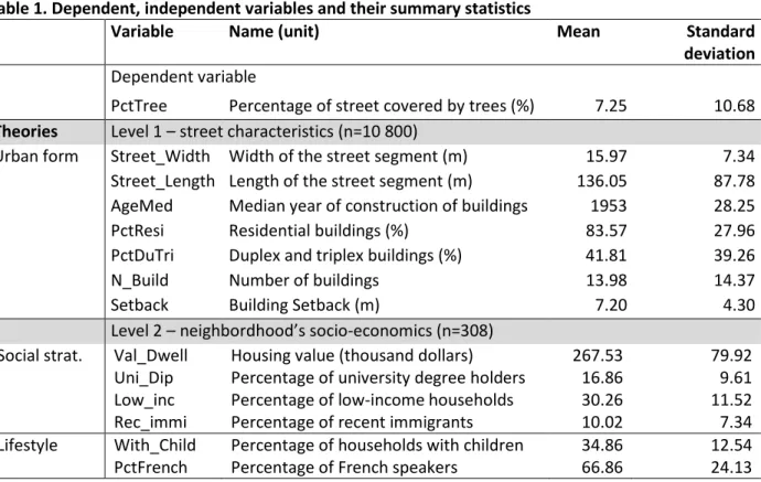
Table 1. Dependent, independent variables and their summary statistics
269
Variable Name (unit) Mean Standard
deviation
Dependent variable
PctTree Percentage of street covered by trees (%) 7.25 10.68
Theories Level 1 – street characteristics (n=10 800)
Urban form Street_Width Width of the street segment (m) 15.97 7.34 Street_Length Length of the street segment (m) 136.05 87.78 AgeMed Median year of construction of buildings 1953 28.25
PctResi Residential buildings (%) 83.57 27.96
PctDuTri Duplex and triplex buildings (%) 41.81 39.26
N_Build Number of buildings 13.98 14.37
Setback Building Setback (m) 7.20 4.30
Level 2 – neighbordhood’s socio-economics (n=308)
Social strat. Val_Dwell Housing value (thousand dollars) 267.53 79.92 Uni_Dip Percentage of university degree holders 16.86 9.61 Low_inc Percentage of low-income households 30.26 11.52 Rec_immi Percentage of recent immigrants 10.02 7.34 Lifestyle With_Child Percentage of households with children 34.86 12.54 PctFrench Percentage of French speakers 66.86 24.13
270
271
Level 1 independent variables – street characteristics
272
We chose urban form variables that were identified in the literature as important correlates of
273
urban vegetation and tree cover. These are: width of the street segment, i.e., street width; length
274
of the street segment, i.e., street length; median age of buildings on the street segment,
275
construction age; percentage of residential buildings; percentage of duplexes and triplexes;
276
number of buildings; and building setback, i.e., setback (Table 1). It is important to note that street
277
width is likely correlated with the type of street, such as arterial, collector or local. Nevertheless,
278
street width was designated as a quantitative physical measurement rather than as one referring
279
to a category of use.
280
Street segments were created from the street map provided by the City of Montréal. To estimate
281
the width and length of street segments, we used the “bounding containers” tool in ArcGIS to
282
measure the two axes of the rectangle that fits the street segment the best. In order to compute
283
the other variables, we joined the street segment map with the parcel and building maps
284
(provided by the City of Montréal). Each parcel and building was associated to one and only one
285
street segment. We then computed the median value of building age per street segment, the
286
average value of the proportion of residential use, commercial use and industrial use; as well as
287
the proportion of duplex, triplex houses by street segment. For each street segment, an average
288
value of building setback was computed. The building setback was defined as the distance
289
between a building and the street, which corresponds roughly to sidewalk width in high density
290
urban areas (Figure 4). These variables do not suffer from multicollinearity problems. Their
291
variance inflation factor (VIF) (Chatterjee & Hadi, 2006) are lower than 2.
292
Figure 4. Illustration of setback of a street in downtown Montréal. Photo credit: first author
293
Level 2 independent variables − neighborhood context
294
To capture effects of neighborhood context on STC, we used the census tracts produced by
295
Statistics Canada (Table 1). We selected a set of variables that proved important in previous tree
296
studies (Bigsby et al., 2013; Grove et al., 2014; Landry & Chakraborty, 2009; Pham et al., 2013;
297
Troy et al., 2007). Exclusion of variables that suffered from multicollinearity was conducted based
298
on the VIF values.
299
Level 2 independent variables related to the social stratification theory are: dwelling value;
300
percentage of university degrees; percentage of recent immigrants (migrating from 1996 and
301
2006); and percentage of low-income households. The percentage of renters was not retained
302
because it is highly correlated with the percentage of low-income households (Pearson r=0.8,
303
VIF=5.03). At Statistics Canada, “low-income households” is a census variable defined as “income
304
levels [before tax] at which families or persons not in economic families spend 20% more than
305
average of their before tax income on food, shelter and clothing” (Statistics Canada 2006: 143). It
306
is worth noting that although recent immigrants are lumped into one variable, we are aware
307
ethnocultural groups may differ greatly in their preferences for vegetation, and some may prefer
308
less or no vegetation (Fraser & Kenney, 2000). Combining all the groups into one category may
309
mask those variations in preferences. However, the low percentage of each group in the total
310
immigrants would prevent a statistically robust analysis.
311
Level 2 variables related to the lifestyle theory included two variables that are relevant to the case
312
of Montréal. First, to characterize the family status, we chose the percentage of families with
313
children instead of the percentage of married couples, as is done in other studies (e.g. Troy et al.,
314
2007). This is because in the province of Quebec, where Montréal is located, only 38% of couples
315
are in common-law relationships but almost 63% of children are born in a common-law
316
relationships (Bourdais et al., 2014). The second variable is the percentage of French speakers as a
317
proxy of cultural and linguistic identities. In Montréal these identities differ among French, English
318
and non-official language speakers. For example, the English-speaking population finds it
319
important to preserve their local community and to express their social and cultural specificity
320
(Boudreau, 2003; Boudreau et al., 2006) through community-building activities, such as high
321
participation in local planning. Differences in identities of these groups can influence locational
322
choices of residence as well as public policies and ordinances related to the environment
323
(Boudreau et al., 2006) and tree protection/planting at the local level (borough, in the case of the
324
City of Montréal). As explained above, we could not introduce each ethnocultural group of the
325
‘non-official language speakers’ in the model. Our models might miss nuances of preferences
326
toward urban trees among these groups.
327
In terms of sample size, researchers have recommended a minimum of five level 1 observations
328
per level 2 group (Maas & Hox, 2005). We removed census tracts that have fewer than five street
329
segments (n=4, or 1.28%). In total, our study area contains 10,800 street segments that are nested
330
in 308 census tracts.
331
Regarding spatial dependency, we determined the radius of the spatial lag term for the models by
332
comparing values of the Moran’s I statistic calculated over the range of 100 to 500 meters. We
333
identified that spatial autocorrelation was maximized at the distance of 200 meters, and therefore
334
computed the spatial lag of STC at this radius.
335
Model specifications
336
We implemented multi-level and mixed models within the R version 3.1.2 environment using the
337
lmerTest package (R Foundation for Statistical Computing, 2015). Models were fitted using
338
restricted maximum likelihood estimation to provide unbiased estimates of variance and
339
covariance parameters (Hox, 1998).
340
We explored several cases of the model by integrating increasing complexity to investigate the
341
role of different model components. In all models we let intercepts vary randomly at the census
342
tract level to account for interdependence among observations. The first of these, Model 1,
343
contained tract-level intercepts only, allowing us to assess variations in STC across census tracts.
344
We expanded this approach to include estimations of coefficients for physical properties of street
345
segments in Model 2, of coefficients for tract-level social stratification variables in Model 3a, and
346
of social stratification and lifestyle in Model 3b. Model 4a considered covariates at the level of the
347
street segment as well as social stratification covariates at the tract level. Model 4b considered all
348
covariates at the street and tract levels. Finally, in Model 5 we introduced all variables of Model 4b
349
and also interactions of four street variables (PctResi, percentage of residential buildings; PctDuTri,
350
percentage of duplexes and triplexes; N_Build, number of buildings; and Setback, building setback)
351
with all the census variables in order to see how these change their effect across different
352
characteristics of streets. All four street variables were considered to be random. Street width,
353
street length and construction age were not included in interactions as we consider them to be
354
control factors.
355
We compared model fits using the Akaike information criterion (AIC) and the Bayesian information
356
criterion (BIC). For Model 1 we also computed the intra-class correlation (ICC), which represents
357
the proportion of between-tract variance in the total variance, as follows:
358
𝐼𝐶𝐶 = 𝜎𝑢2/(𝜎𝑢2+ 𝜎𝑒2) [1]
359
where the variance parameters 𝜎𝜇2 and 𝜎𝑒2 represent the within-tract and between-tract variances,
360
respectively.
361
ICC indicates the proportion of the variance of the dependent variable explained by unaccounted
362
for census tract-level heterogeneity.
363
RESULTS
364
Effects of the three theories on STC
365
Moran’s I tests on residuals of the models with and without the spatial lag show that models
366
without the spatial lag suffer from the spatial autocorrelation problems as Moran’s I on their
367
residuals varying from 0.12 to 0.17. Models that included the spatial lag variable produce residuals
368
that are not spatially correlated with Moran’s I varying from −0.02 to 0.05. This confirms the need
369
to test spatial autocorrelation and introduce a spatial term in the models.
370
Fixed and random effects of the first four models are shown in Table 2. The spatial lag is significant
371
in all models. AIC indicators indicated that Model 2 (including only street variables; 77,752.50) was
372
better than Model 3a (79066.5) and Model 3b (including only tract variables; 79,062.10). Model 2
373
was even slightly better than Model 4a (77,760.20) and 4b (77,756.80). Comparing Model 3a and
374
3b, and Model 4a and 4b, lifestyle variables result in a slightly lower AIC, suggesting that these
375
variables contribute to explaining the variation of STC, albeit to a small degree.
376
Table 2. Fixed and random effects of the four models without interactions
378
Model 1 Model 2 Model 3a Model 3b Model 4a Model 4b
Theories Fixed effects
β t-value β t-value β t-value β t-value β t-value β t-value Urban form Intercept 7.38 26.46 *** -6.21 -12.54 *** 0.73 1.64 -0.84 -0.62 -7.17 -10.37 *** -8.10 -5.53 ***
Street_Width -0.11 -9.04 *** -0.11 -9.28 *** -0.12 -9.44 *** Street_Length 0.01 6.45 *** 0.01 6.38 *** 0.01 6.38 *** PctDuTri 0.00 -2.03* 0.00 -1.88 -0.01 -2.29* PctResi 0.04 12.52 *** 0.04 12.39 *** 0.04 12.47 *** AgeMed 0.06 8.02 *** 0.06 7.72 *** 0.05 7.52 *** AgeMed2 0.00 -4.62 *** 0.00 -4.64 *** 0.00 -4.46 *** N_Build 0.13 13.52 *** 0.13 13.46 *** 0.14 13.54 *** Setback 0.18 8.55 *** 0.18 8.19 *** 0.18 8.25 *** Spatial lag 0.69 44.28 *** 0.80 50.53 *** 0.79 49.38 *** 0.67 41.40 *** 0.67 41.54 ***
Social strat. Val_Dwell 0.00 1.86 0.00 3.03 ** 0.00 2.43 ** 0.01 4.05 ***
Uni_Dip 0.02 1.95 0.01 0.79 0.02 1.54 -0.01 -0.45 Low_inc -0.02 -2.06* -0.03 -2.07* -0.01 -1.03 -0.03 -1.82 Rec_immi 0.03 1.75 0.07 3.05 ** 0.03 1.61 0.08 3.74 ** Lifestyle With_Child 0.00 -0.18 -0.02 -1.50 PctFrench 0.02 2.28* 0.02 2.59 ** AIC 80193.10 77752.50 79066.50 79062.10 77760.20 77756.80 BIC 80200.50 77760.00 79092.60 79095.70 77767.60 77764.30 Random effects Intercept - Census tract 19.89 0.55 0.00 0.00 0.4573 0.31 Residuals - Street 93.01 77.40 88.51 88.44 77.3206 77.31 ICC 0.18 *** p < 0.001; ** p < 0.01, *p<0.05
379
The introduction of street characteristics of the urban form reduced both the variance of STC at
380
the tract level (between-tract variance reduced from 19.89 in Model 1 to 0.55 in Model 2) and the
381
variance at street level (from 93.01 in Model 1 to 77.40 in Model 2). The introduction of social
382
stratification and lifestyle variables substantially reduced variance at the tract level, from 19.88 to
383
0.00 in Model 3a and 3b, yet not at the street level. This is understandable because street-level
384
variables can explain variation of STC at the tract level but not inversely. This suggests that street
385
variables of the urban form are more efficient in explaining street-level variations of STC, but that
386
social stratification and lifestyle variables are more efficient in explaining tract-level variations of
387
STC. Overall, at both levels, street variables of the urban form are more important than social
388
stratification and lifestyle variables in explaining STC.
389
Model 1: Variation explained by differences between neighborhoods
390
The ICC indicates that between-tract variance can explain up to 17.6% of the total variance. This
391
suggests that political, socio-economic or other explanatory factors operating at the tract level and
392
relating to STC can potentially explain 17.6% of the variation of tree cover.
393
Model 2: Variation explained by street characteristics
394
Accounting for street-level urban form covariates (Table 2), all variables are significant at p<0.01.
395
The most significant variable is number of buildings (N_Build, t-value=13.52), with STC increasing
396
as the number of buildings increases. The second important variable is percentage of residential
397
buildings on the street, with a positive association (t-value=12.52). This suggests that a residential
398
street tends to have larger STC than industrial or commercial streets. Not surprisingly, street width
399
has a negative and significant association with STC (t-value=−9.04), meaning that the surfaces of
400
wide streets tend to be less covered by trees. This is due to two facts. First, wider streets are less
401
likely to have nearby tree canopy large enough to cover a large proportion of the street surface.
402
Second, wide streets tend to be arterials, which generally have fewer trees.
403
Setback, the distance between a building and the street, has a strong and significant positive
404
association with tree cover (t-value=8.55): STC is greater on streets with a wider setback. Street
405
length also has a positive association with tree cover (t-value=6.45), meaning that STC is greater
406
on longer streets. The two variables concerning the construction age are significant, suggesting
407
that the relationship between construction age and STC was U-shaped. Finally, percentage of
408
duplexes and triplexes is negatively associated with STC (t-value=−2.03), suggesting that streets
409
having these types of buildings have less STC.
410
Model 3a and 3b: Variation explained by social stratification and lifestyle
411
In Model 3b, dwelling value is positively significant (t-value=3.03), meaning streets with more
412
expensive houses tend to have more STC. The percentages of recent immigrants and of French
413
speakers have a positive coefficient (t-value=3.05 and 2.28, respectively). Even after controlling for
414
these variables, the percentage of low-income households still has a negative association with STC
415
at p<0.05 (t-values=−2.07).
416
Models 4a and 4b: Variation explained by street characteristics as well as context
417
In Model 4a and 4b, variable coefficients change slightly compared to the previous models.
418
Variances of errors in random effects are much lower than those in the previous models,
419
suggesting that combining variables at the two levels is more helpful in explaining variations of
420
STC.
421
Model 5: Interactions between the street characteristics and context variables
422
Results of the interactions in Model 5 are reported in Table 3. Only significant variables are shown
423
due to lack of space. The AIC value (77,578.8) is lower here than in all other models, suggesting
424
that the inclusion of the interactions contributed to explaining STC. At the street level, street
425
width, street length, percentage of duplexes and triplexes as well as construction age are
426
significant with similar coefficients of Model 2. However, three street variables become
non-427
significant (percentage of residential buildings, number of buildings, and setback), although some
428
of their interactions remain significant. At the neighborhood level, the only significant variable is
429
the percentage of French speakers.
430
Table 3. Fixed and random effects Model 5 (with interactions)
431
Variables β t-value
Fixed effects
Street level Street_Width -0.1149 -9.55 ***
Street_Length 0.008601 5.14 ***
PctDuTri -0.09314 -2.66 **
AgeMed 0.04976 6.90 ***
AgeMed2 -0.00017 -3.89 ***
Spatial lag 0.5162 29.50 ***
Census level French -0.05973 -2.48*
Interactions PctResi *Val_Dwell 0.000143 2.73 ** PctResi * Rec_immi 0.001518 2.24* PctResi *French 0.000504 2.17* N_Build * Low_inc -0.00460 -3.14 ** N_Build * Rec_immi 0.006673 2.90 ** N_Build *With_Child -0.00403 -2.63 ** PctDuTri *Uni_Dip 0.000926 2.31* PctDuTri * Low_inc 0.000731 2.18* Setback*Uni_Dip 0.01286 2.95 ** AIC 77578.8 BIC 77597.4 Random effects
PctResi – Census tract 0.000037 N_Build – Census tract 0.01428 PctDuTri – Census tract 0.000022
432
433
We plotted the amount of STC against each socio-demographic variable by using coefficients
434
estimated from Model 5 (Fig. 5). The plots were created separately for three types of census tracts
435
according to their differences in street characteristics. For example, census tracts are considered
436
as having a “low residential level” when the standard deviation of PctResi (percentage of
437
residential buildings) is subtracted from the mean value of this variable; a “medium residential
438
level” when PctResi equals the mean value of this variable; and a “high residential level” when the
439
standard deviation of PctResi is added to the mean value of this variable.
440
441
Figure 5. Effects of socio-demographic factors across different levels of street characteristics
442
443
The most influential interaction takes place between dwelling value and percentage of residential
444
buildings on the streets, indicating that STC is higher in expensive areas having highly residential
445
streets. STC is also higher in areas inhabited by recent immigrants on highly residential streets. STC
446
is slightly lower in French-speaking areas having a lot of residential buildings on the streets.
447
STC is lower in areas that are inhabited predominantly by low-income households and by families
448
with children, and that have a large number of buildings. Inversely, STC is higher in areas with a
449
high percentage of recent immigrants and on streets having a large number of buildings. STC is
450
also higher in areas inhabited predominantly by low-income households and by university degree
451
holders in duplexes and triplexes. The only variable that has a significant interaction with setback
452
Setback – Census tract 0.007152 Residuasl - street 71.3397
is the percentage of university degrees. STC is higher in areas with high levels of education, and the
453
effect is stronger in streets with a larger setback.
454
DISCUSSION
455
In this paper, we examined the roles of physical street characteristics and neighborhood context
456
on the variation of street tree cover (STC) using two-level and mixed models. We used fine-grained
457
data on street characteristics that allowed us to capture associations between STC and the urban
458
form. Furthermore, the use of mixed effects, a spatial term and interactions in our models allowed
459
us to obtain more robust results. In this section, we will focus on the results of the last and the
460
most complex model, Model 5, because it was the best performing (lowest AIC) and contained the
461
most information.
462
Street characteristics and the urban form
463
All our model results indicate that the variables representing the urban form are more important
464
than those representing social stratification and lifestyle. While the number of buildings has a
465
positive association with STC, the percentage of duplex and triplex housing,(which tends to be high
466
in dense and central quarters in Montréal, has a negative association with STC. Our findings with
467
respect to housing types are similar to previous research, which found higher canopy cover in
468
areas with a higher proportion of single-family homes (Troy et al., 2007). A possible explanation
469
for these findings is tenure modes. Nowak et al. (1990) observed that homeowners, more likely to
470
live in single-family homes, are more likely to engage in the care of street trees than renters who
471
are more likely to live in duplex and triplex houses.
472
Street width has a negative association with tree cover. Although street width is partially
473
confounded here with types of streets, for example arterials are wider than local streets, STC was
474
likewise lower on wider streets. One possible explanation is that the City did not prioritize planting
475
trees along arterials that are not used for walking. To verify this explanation, interviews with the
476
City are needed, which is beyond the scope of this study. Another plausible explanation is that
477
trees are sparsely planted on big streets in order to reserve space for facilities such as power lines
478
and drainage systems, or that trees are restricted by transport engineering standards in order to
479
maintain clear zones for traffic safety (Wolf & Bratton, 2006). The construction age has a U-shaped
480
relationship with tree cover, which corroborates previous studies on urban vegetation (Grove et
481
al., 2006; Landry & Chakraborty, 2009; Mennis, 2006).
482
483
Socio-demographic context and its interactions with street characteristics
484
The introduction of socio-demographic variables helps increase the proportion of explained
485
variance of STC at the tract level. Lifestyle variables prove to be important in explaining STC due to
486
the percentage of French speakers, although much less so than social stratification variables.
487
Street characteristics interact very differently with socio-demographic variables. For example,
488
percentage residential has a positive interaction with dwelling values and with percentage of
489
recent immigrants, but a negative interaction with percentage of French speakers. Number of
490
buildings on the streets also has different interactions with socio-demographic variables: positive
491
interactions with recent immigrants and negative interactions with low-income households as well
492
as with families with children. This means that STC is lower in areas having a high number of
493
buildings and inhabited by the last two groups. Given the economic situation and health status of
494
the latter two groups, these results might raise environmental equity concerns that highlight a
495
greater need for tree cover.
496
Interestingly, some socio-demographic variables have different effects from one model to another.
497
In the models without interaction, percentage of low-income households is negatively associated
498
with STC. In the interactive model, this variable interacts negatively with the number of buildings
499
but positively with the percentage of duplexes and triplexes. The percentage of French speakers
500
has positive effects in the non-interactive models but negative effects in the interactive model.
501
Explaining why STC is lower in French-speaking areas having a lot of residential buildings needs
502
further research. Even if the reasons for these relationships are (still) unclear, these findings
503
highlight the importance of the urban form when considering the relationship between social
504
stratification and STC.
505
Three social stratification variables that do not change the direction of their coefficients across
506
models are dwelling value, recent immigrants and university degrees, and all three have positive
507
associations with STC. When interacting with the residential variable at the street level, dwelling
508
values and recent immigrants have positive interactions in streets having a high number of
509
residential houses. It is suggested in the literature that residential streets have favorable growing
510
conditions for trees because water and nutrients from residential front yards are more likely to be
511
close to street tree planting pits. Moreover, as residential streets are less exposed to car and
512
pedestrian flows, trees there are less likely to become damaged and vandalized (Jim, 1987; Nowak
513
et al., 1990). The interaction results suggest that in Montréal the influence of the number of
514
residential houses on STC is even higher in expensive neighborhoods. This finding would support
515
the social stratification explanation, in that one might expect the differential influence on tree
516
planting associated with socio-economic status to be greater in areas where people live.
517
The percentage of recent immigrants has a positive association with STC, as exemplified with the
518
Côte-des-Neiges and Loyola neighborhoods (marked as 1 and 2 on Figure 2). Côte-des-Neiges,
519
being an older neighborhood with an aging housing stock, was designed in keeping with the urban
520
form principles of the time (mostly constructed before World War II and in the 1950s), which
521
allowed for a high STC. It is usually chosen by new arrivals and university students because of its
522
affordable housing stock, proximity to colleges and universities, abundant public services, such as
523
hospitals and available community support. In 2006, 54% of its population is immigrants, mostly
524
from Asia (Southeast Asia in particular) and North Africa. Of these, more than one third was recent
525
immigrants (INRS-UCS, 2010a). As for Loyola, recent immigrants also made up one third of its
526
immigrant population. Immigrants were principally from Europe (notably Eastern Europe) and Asia
527
(Eastern Asia in particular) (INRS-UCS, 2010b). In this neighborhood, it is common to find detached
528
houses and high-rise buildings on the same street. High-rise buildings are often chosen by recent
529
immigrants for their lower price. Detached houses with gardens and well-vegetated streets
530
contribute largely to the greenness of the neighborhood.
531
We also found positive associations between STC and high dwelling value, especially in highly
532
residential streets and university degree. These suggest that households with limited housing
533
budgets and less education tend to live in neighborhoods with a small amount of STC and with less
534
of the benefits provided by street trees. This lack of environmental equity of STC is likely
535
attributed to several mechanisms. The first mechanism is related to the social-stratification
536
explanation of uneven STC distributions related to purchasing power: green and tree-shaded
537
neighborhoods are more expensive (Donovan & Butry, 2010). The second mechanism concerns
538
differences in the motivation behind greening initiatives of neighborhood-based organizations and
539
individuals associated with socio-economic status. A study conducted in Missouri shows that
540
residents from high-income and high-education areas were more willing to fund street tree
541
programs (Treiman & Gartner, 2006). In Montréal, residents do not fund tree programs but they
542
have an influence on where municipal funds are going, especially by exerting pressure on their
543
municipal counselors which are elected every four years. Further contrasting reactions to tree
544
planting were observed in Hobart (Australia), where poor neighborhoods had a hostile reception
545
of new plantings, even to the point of destroying them; while wealthy suburbs exhibited no signs
546
of objection (Kirkpatrick et al., 2011).
547
CONCLUSION
548
In this paper, we were able to capture the variations of STC explained by each of the three
549
theories (urban form, social stratification and lifestyle). All three prove to be important in
550
explaining STC, whereby urban form proved to be the most essential, followed by social
551
stratification and lifestyle. Some interactions between street characteristics and
socio-552
demographic variables are significant, suggesting that interactions merit further examination in
553
future studies on urban forests. The interactions observed in this study could be used to better
554
design greening strategies taking into account both the urban form and socio-demographic
555
context. Empirical evidence from Montréal in this paper contributes to enrich and enlarge
556
theoretical frameworks of STC correlates. However, the development, application and
557
interpretation of the models are complex. The selection of variables was made carefully while
558
taking into consideration our knowledge about the study area. Methodology in this paper could be
559
used to model urban tree cover in other cities. The choice of variables and results will depend on
560
physical and socio-demographic particularities of the cities.
561
Our findings provide insight for urban planners to address possible inequities in the distribution of
562
street trees in order to increase tree cover and reduce heat islands in problematic areas of the
563
city. For example, the careful design of tree planting along wide streets could enhance road safety,
564
and a greater number of trees on commercial streets could render those streets more walkable
565
and livable. In Montréal, where public trees are usually planted on sidewalks, sidewalks in new
566
neighborhoods should be designed wide enough so that trees can grow adequately. In dense areas
567
where wider sidewalks are not possible, urban planners could resort to alternatives such as green
568
roofs or green walls. However, such greening measures might be inferior to trees in terms of their
569
ecosystem value.
570
Our paper also reveals that high dwelling value and high level of education were associated with
571
more STC, while low-income areas tend to have lower STC, even after controlling for the urban
572
form. These results point to the need to integrate local equity in greening programs. More
573
importantly, greening should be done in a way that avoids creating or exacerbating concerns
574
about environmental inequity. In other words, equity should be a key principal in urban forest
575
programming. Evidence from other cities has shown that greening efforts may create paradoxical
576
effects on equity. Urban planners, local stakeholders, communities and gentrifiers need to
577
collaborate in the planting of trees. They can do so by resisting speculative development, targeting
578
areas inhabited by low-income families, encouraging participative planning, and prioritizing
small-579
scale sites over grand green projects (Wolch et al., 2014). Other strategies can be also useful, such
580
as raising public awareness and informing local residents about plantings and procedures.
581
582
REFERENCES