1
This is an accepted manuscript of an article published by Elsevier in Applied Geography on Septembre 24 2016, available at http://dx.doi.org/10.1016/j.apgeog.2016.09.023
This manuscript version is made available under de CC-BY-NC-ND 4.0 license http://creativecommons.org/licenses/by-nc-nd/4.0/
Please cite as:
Apparicio, Philippe, Thi-Thanh-Hien Pham, Anne-Marie Séguin, and Jean Dubé. 2016. "Spatial distribution of vegetation in and around city blocks on the Island of Montreal: A double environmental inequity?"
2
Spatial distribution of vegetation in and around city blocks on the Island of
1Montreal: a double environmental inequity?
2Abstract
3
Recent studies have shown that urban vegetation is unevenly distributed across numerous North American cities: 4
neighbourhoods predominantly inhabited by low-income populations and/or by certain ethnic groups have less 5
vegetation cover. The goal of this paper is to examine the existence of environmental inequities related to access 6
to urban vegetation on the Island of Montreal for four population groups (low-income people, visible minorities, 7
individuals 0-14 years old and persons 65 years old and over). Six indicators of vegetation in and around 8
residential city blocks (within 250 m and 500 m) are computed by using QuickBird satellite images. These 9
indicators are then related to socioeconomic data by using different statistical analyses (T-test, seemingly 10
unrelated regression and multinomial logistic regression). The results show that low-income people and, to a 11
lesser degree, visible minorities reside in areas where vegetation is less abundant. On the other hand, the 12
opposite situation is found for children and the elderly. The use of indicators computed in and around city blocks 13
leads to the finding of a double inequity in certain neighbourhoods. This points to the need to target vegetation-14
deprived areas for urgent greening in order to improve vegetation cover within city blocks (in residential yards 15
or through alternatives such as green walls and green roofs) and around these blocks (along streets and in parks). 16
17
Keywords: urban vegetation; environmental equity; environmental justice; spatial analysis; remote sensing;
18
seemingly unrelated regression; Montreal. 19
20 21
3
1. Introduction
22
Most large cities around the world have acknowledged the crucial role of nature in the city. North American 23
cities are no exception: they have recognized the important part that urban vegetation plays in the quality of life 24
by implementing tree preservation and tree planting measures in both the United States (Hubacek & Kronenberg, 25
2013) and Canada (City of Montréal, 2011; City of Toronto, 2013). Moreover, the many benefits of urban 26
vegetation have recently been documented, on the biophysical, health, social and economic levels. Numerous 27
studies have shown that vegetation helps to improve the quality of the urban environment by reducing air and 28
noise pollution, capturing a portion of the carbon in the air, helping to save energy, and, more vitally, 29
minimizing the negative impacts that heat islands have on the health of populations (Mullaney, Lucke, & 30
Trueman, 2015; Roy, Byrne, & Pickering, 2012). In terms of people’s well-being and social benefits, a number 31
of authors from various disciplines note that the presence of vegetation helps to lower stress levels and 32
contributes to the social integration of the elderly, children and adolescents, especially in multiethnic urban areas 33
(de Vries, van Dillen, Groenewegen, & Spreeuwenberg, 2013; Taylor, Wheeler, White, Economou, & Osborne, 34
2015). Finally, on the economic level, other scholars emphasize that vegetation can be profitable for cities 35
(Mullaney, et al., 2015), for example by reducing electricity consumption and increasing property values 36
(Donovan & Butry, 2010). 37
Several recent studies have however shown that urban vegetation is not equitably distributed across North 38
American cities, to the detriment of certain population groups such as low-income households and visible 39
minorities (e.g. Landry & Chakraborty, 2009; Pham, Apparicio, Séguin, Landry, & Gagnon, 2012; Schwarz, et 40
al., 2015; Tooke, Klinkenberg, & Coops, 2010). These studies frequently use high resolution satellite images 41
(e.g. QuickBird, Ikonos imagery, etc.) to build vegetation indicators, spatial census data integrated into 42
Geographical Information Systems (GIS) and statistical methods to explore the associations between vegetation 43
indicators and socioeconomic variables. The approach taken here is in line with this type of studies: its objective 44
is to verify the existence of environmental inequities regarding access to urban vegetation on the territory of the 45
Island of Montreal for the four population groups most often examined in studies on environmental equity: that 46
is, low-income populations, visible minorities, children and the elderly. The article focuses in particular on 47
access to vegetation within residential city blocks, as well as around these blocks, in order to determine whether 48
some groups are more likely to be affected by a double inequity than others. 49
The study attempts to answer three research questions. The first question is: Where are the areas located that 50
have little vegetation both in and around the city block, and, conversely, that have a large amount of vegetation 51
in and around the city block? The second question is: Do children, seniors, low-income populations and visible 52
minorities live in areas with little vegetation in and around their city block? The third question is: After 53
4
controlling for the characteristics of the built environment (population density and age of the neighbourhoods), 54
do the four population groups studied live in residential areas with proportionately more or less vegetation? 55
The paper is organized as follows. It begins by discussing the notion of environmental equity as applied to urban 56
vegetation, in emphasizing the use of vegetation indicators on a number of scales. It then describes the 57
methodological approach taken in this study, which combines multisource data (satellite images, GIS data from 58
the City of Montreal and census data) and various methods from the fields of GIS, remote sensing, and spatial 59
analysis. After this, a concise presentation of the results is followed by a discussion of the findings. 60
2. Literature review
61
Walker (2012) identifies and defines three dimensions of environmental justice: distributive justice, procedural 62
justice and justice as recognition. The first is understood in terms of the distribution or sharing of beneficial 63
elements (resources) and negative elements (sources of risk). The second dimension refers to the ways that 64
decisions are made, who is involved, and who has the power to influence such decisions. The third is based on 65
the idea of respect for all individuals in a given society and rejects the manifestation of disrespect toward 66
particular social groups. Environmental justice thus recognizes that all individuals in a given society, regardless 67
of their status, have the right: 1) to live in a healthy environment with access to basic territorial resources; and 2) 68
to participate in the process of formulating laws, policies and environmental regulations. 69
This study is interested in the first dimension: that is, environmental equity or distributive justice. Several studies 70
carried out in North America and based on different methodologies have demonstrated the existence of 71
environmental inequities in terms of access to vegetation for low-income populations (Heynen, 2006; Landry & 72
Chakraborty, 2009; Pham, et al., 2012; Tooke, et al., 2010). In Canada, Tooke, et al. (2010) find that the amount 73
of vegetation is negatively associated with the percentage of low-income persons per census tract, whereas it is 74
positively associated with median and average incomes for both individuals and households, in Montreal, 75
Toronto and Vancouver. However, the correlation between the percentage of immigrants and the amount of 76
vegetation is only negatively significant in Toronto. In Montreal, Pham, et al. (2012) conclude that low-income 77
populations and, to a lesser degree, visible minorities, live in city blocks where there is less vegetation on 78
average. In the United States, the results are however less conclusive for racial minorities. In Tampa, Landry and 79
Chakraborty (2009) show that, the percentage of tree cover on streets declines as the proportions of African-80
American and Hispanic residents rise. In Baltimore and Milwaukee, on the other hand, African Americans do 81
not seem to have more limited access to vegetation, unlike the case for Hispanic residents (Heynen, 2006; Troy, 82
Grove, O'Neil-Dunne, Pickett, & Cadenasso, 2007). 83
Many studies on environmental equity and vegetation look at vegetation within city blocks or census block 84
groups (Landry & Pu, 2010; Pham, Apparicio, Landry, Séguin, & Gagnon, 2013; Pham, et al., 2012; Troy, et al., 85
5
2007). This spatial approach, although interesting, leaves room for improvement. An individual may in fact live 86
in a block with largely impervious surfaces—in other words, in a block with little vegetation—whereas there is a 87
large amount of vegetation cover around that block, and vice versa. For example, a person may live in a block 88
with very little vegetation, primarily consisting of high-density housing, but that faces a large park. On the other 89
hand, little vegetation in the immediate environment around the residential block would represent a double 90
disadvantage. In other words, evaluating the existence of vegetation cover should not be spatially limited to the 91
block where the person lives, but should also include the immediate environment around the block. Indeed, if, 92
compared with the rest of the population, a population group is overrepresented in spaces with little or no 93
vegetation both in and around the residential city block, this constitutes a double environmental inequity. 94
Because some authors (Bowen, 2002; Cutter, Holm, & Clark, 1996) have emphasized the relevance of 95
examining exposure to nuisances or access to benefits on a number of spatial scales (e.g. census tracts, block 96
groups, census blocks, buffer zones), this study uses a method of evaluating distributional inequity that involves 97
measuring the access to vegetation on several scales: within the city block, and within 250 and 500 metres 98
around the residential block. 99
In environmental equity studies related to the distribution of vegetation, it has been shown that the presence of 100
vegetation is negatively associated with residential density and the age of the built environment (Grove, et al., 101
2006; Landry & Chakraborty, 2009; Mennis, 2006; Pham, et al., 2013; Pham, et al., 2012). In the case of the 102
Island of Montreal, low-income populations and visible minorities are concentrated in central City of Montreal 103
neighbourhoods that often have the highest residential densities and an older built environment (Séguin, 104
Apparicio, & Riva, 2012). Conversely, young children are more often found in suburban municipalities with a 105
recent built environment and low residential density. The elderly, on the other hand, are concentrated both in 106
central neighbourhoods and in the first-ring suburbs of the Island of Montreal (Séguin, Apparicio, & Riva, 107
2015). It is therefore appropriate to control for these two characteristics of the built environment in order to 108
arrive at an accurate environmental equity assessment. 109
3. Study area and methodology
110
The study covers the territory of the municipalities on the Island of Montreal, which extends over roughly 500 111
km2 and included 1.85 million inhabitants in 2006. This territory is the central part of the Montreal census 112
metropolitan area (CMA), which is the second most populous metropolis in Canada (with 3.92 million 113
inhabitants). 114
3.1. Data processing
115
To answer the research questions, two sets of data were employed. QuickBird images (acquired in September 116
2007, 60 cm resolution) were used to map two types of vegetation, that is, trees/shrubs and grass/lawn, based on 117
6
an object-oriented classification performed in e-Cognition (Pham, Apparicio, Séguin, & Gagnon, 2011); and 118
socioeconomic data were extracted from the 2006 census on the level of the dissemination area. 119
It was then a matter of defining the spatial entities in which the socioeconomic and vegetation indicators would 120
be calculated. As several other authors had done (Pham, et al., 2013; Pham, et al., 2012), we selected the finest 121
spatial division, that is, the city block. Two buffer zones were defined around the block within a radius of 250 122
and 500 metres, excluding the block itself. The second step was to build the six vegetation indicators: the 123
proportions of the surface area of the block that were completely covered by total vegetation (trees/shrubs and 124
grass/lawn) and by trees/shrubs alone; the proportions of the surface area of the buffer zones of 250 and 500 125
metres around the block that were covered by total vegetation and by trees/shrubs. These two distances were 126
chosen in order to define immediate environments that can easily be reached on foot. These two distances have 127
moreover already been used in Montreal in studies on the accessibility of services (Apparicio, Abdelmajid, Riva, 128
& Shearmur, 2008; Apparicio, Séguin, & Naud, 2008). 129
The third step was to bring the numbers of the four groups studied —children under age 15, people aged 65 and 130
over, the population with low income before tax, and visible minorities1—extracted from the 2006 census down 131
to the level of city blocks. It should be noted that the only three variables available from Statistics Canada on the 132
scale of the dissemination block (i.e. city block) were the total population, the number of households and the 133
number of occupied dwellings. To bring the data available on the level of the dissemination area (DA, i.e. city 134
block group in the United States), that is, a spatial area larger than that of the city block, down to the city block 135
level, a population-based weighting technique, as proposed by Pham et al. (2012), was used. For example, to 136
bring the number of children under age 15 from the DA level down to the city block level, the number of 137
children in the DA in which the block was located was multiplied by the total population of the block divided by 138
the total population of the DA: 139 DA Block DA Block TotalPop TotalPop Pop Pop014 014 [1] 140
3.2. Measuring environmental inequity: Mapping and statistical analyses
141
To answer the first research question—locating areas with little vegetation both in and around the city block—a 142
mapping technique is used based on a cross tabulation composed of the quintiles of two vegetation indicators 143
(the percentage of vegetation in the block and within 250 metres around the block). A typology of the blocks can 144
then be developed according to the various possible combinations between the quintiles of the two variables. For 145
1 According to Statistics Canada, “Visible minority refers to whether a person belongs to a visible minority group as defined by the
Employment Equity Act and, if so, the visible minority group to which the person belongs. The Employment Equity Act defines visible minorities as ‘persons, other than Aboriginal peoples, who are non-Caucasian in race or non-white in colour.’ The visible minority population consists mainly of the following groups: Chinese, South Asian, Black, Arab, West Asian, Filipino, Southeast Asian, Latin American, Japanese and Korean” (Statistics Canada, 2010: 104-105).
7
example, blocks in the fifth quintile for the two indicators are characterized by the highest level of vegetation in 146
and around the city blocks. Conversely, blocks in the first quintile for the two indicators have little vegetation 147
both in and around the city block. With this technique, it is thus possible to identify sectors with a large amount 148
of vegetation within the blocks, but little around the blocks, and vice versa. 149
Three types of statistical analyses are used to answer questions 2 and 3, and, more specifically, to evaluate the 150
statistical relationships between the variables pertaining to the four groups studied and the six vegetation 151
indicators (the univariate statistics for these can be found in Table 1). To answer the second question, we 152
compare the means of the vegetation indicators for the 10,210 blocks weighted by the numbers of the population 153
of each group with the rest of the population (for example, the population under age 15 compared with the 154
population aged 15 and over). The Student’s T-test, widely used in environmental equity studies (Briggs, 155
Abellan, & Fecht, 2008; Carrier, et al., 2016; Carrier, Apparicio, Séguin, & Crouse, 2014a, 2014b), makes it 156
possible to determine whether the four groups studied live in environments with significantly less vegetation 157
than is the case for the rest of the population. 158
To answer question 3, regression models are used. As mentioned above, the population density and age of the 159
neighbourhoods should be taken into account in equity analyses related to vegetation. Once these two 160
characteristics have been controlled for in a regression model, this will show whether there are still significant 161
associations between the vegetation indicators and the proportions of the four groups studied. It should be noted 162
that the median age of the residential buildings in the blocks is also introduced in a squared form, as several 163
authors (Grove, et al., 2006; Mennis, 2006; Pham, et al., 2012) have shown that this variable has a curvilinear 164
relationship with the vegetation indicators. Also, for reasons of normality, the population density variable 165
(inhabitants per hectare in the block) has been introduced in logarithmic form. 166
The first type of regression used is a seemingly unrelated regression (SUR). Four models in R (version 3.1.2) are 167
built with the systemfit library (Henningsen & Hamann, 2015). A particularity of this model is the fact that the 168
two equations are estimated simultaneously in order to express: the percentage of the surface area of the block 169
covered by total vegetation or by trees/shrubs (y1); and the percentage of total vegetation or trees/shrubs in buffer
170
zones of 250 and 500 metres around the block, excluding the block itself (y250 ory500), where y is a dependent
171
variable vector of dimension (N × 1), with N being the total number of blocks analyzed (10,210). The model 172
assumes that the two dependent variables (y1 and y250 or y500) are related to two distinct sets of explanatory
173
variables: one set of variables describing the built environment in the block (X1) and the built environment
174
within a 250 or 500 metre radius (X250 orX500); and another set of variables relating to the proportion of the four
175
groups studied in the total population living in the block (X2) (equations 2 and 3).
176
𝑦1 = 𝛼1+ 𝑋1𝛽1+ 𝑋2𝜃1+ 𝜀1 [2]
8
𝑦250= 𝛼2+ 𝑋250𝛽250+ 𝑋2𝜃2+ 𝜀2 or𝑦500 = 𝛼2+ 𝑋500𝛽500+ 𝑋2𝜃2+ 𝜀2 [3] 178
Where the matrices of the explanatory variables, X1, X250 or X500 and X2, are, respectively, of dimensions (N × 3),
179
(N × 3) and (N × 4) and where the parameters of interest (to be estimated) of the built environment β1, β250 and 180
β500 are of dimensions (3 × 1) and those of population groups θ1, θ2 are of the dimensions (4 × 1). The 181
parameters α1 and α2 represent the intercepts and ε1 and ε2 represent the vectors of the error terms of the
182
dimensions (N × 1). A system of equations was chosen since authors such as Zellner (1962, 1963) have shown 183
that when the equations are interrelated via the correlation of the error terms and the explanatory variables in the 184
two equations are different, the coefficients estimated by means of independent equations are biased and the 185
estimated variance-covariance matrix is inaccurate, which thereby invalidates the tests of significance of the 186
parameters. For this reason, and especially to take into account the fact that the relationships are implicitly 187
interlinked, the model is estimated by using seemingly unrelated regression (SUR). 188
Finally, another type of regression is used: that is, multinomial logistic regression with, as the dependent 189
variable, the different types of blocks qualified according to the abundance of vegetation in the block and around 190
the block (as identified by the mapping technique mentioned above). The percentages of each of the four 191
population groups and the variables relating to the built environment in and around the block are introduced as 192
independent variables. This will make it possible to see whether the percentages of each of the four population 193
groups increase the probability of residing in a particular type of block. 194
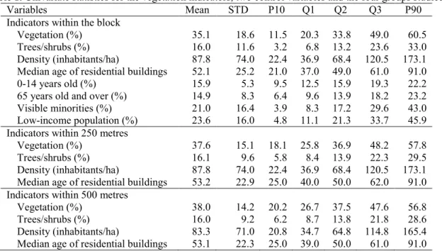
Table 1. Univariate statistics for the vegetation indicators, two control variables and the four groups studied.
195
Variables Mean STD P10 Q1 Q2 Q3 P90
Indicators within the block
Vegetation (%) 35.1 18.6 11.5 20.3 33.8 49.0 60.5
Trees/shrubs (%) 16.0 11.6 3.2 6.8 13.2 23.6 33.0
Density (inhabitants/ha) 87.8 74.0 22.4 36.9 68.4 120.5 173.1 Median age of residential buildings 52.1 25.2 21.0 37.0 49.0 61.0 91.0 0-14 years old (%) 15.9 5.3 9.5 12.5 15.9 19.3 22.2 65 years old and over (%) 14.9 8.3 6.4 9.6 13.9 18.2 23.2 Visible minorities (%) 21.0 16.4 3.9 8.3 17.2 29.6 43.0 Low-income population (%) 23.6 16.0 4.8 11.1 21.3 33.7 45.9
Indicators within 250 metres
Vegetation (%) 37.6 15.1 18.1 25.8 36.9 48.2 57.8
Trees/shrubs (%) 16.1 9.6 5.8 8.4 13.9 22.3 29.5
Density (inhabitants/ha) 87.8 74.0 22.4 36.9 68.4 120.5 173.1 Median age of residential buildings 53.2 22.9 25.0 40.0 50.0 62.0 91.0
Indicators within 500 metres
Vegetation (%) 38.0 14.2 20.2 26.7 37.5 47.6 56.8
Trees/shrubs (%) 16.0 9.2 6.2 8.7 13.8 21.8 28.6
Density (inhabitants/ha) 83.3 71.0 20.8 34.7 64.8 114.8 165.4 Median age of residential buildings 53.1 22.3 25.0 39.0 50.0 61.0 91.0
N = 10,210. STD: standard deviation; P10: 10th percentile; Q1: lower quartile; Q2: median; Q3: upper quartile; P90: 90th percentile.
196 197
9
4. Results
198
4.1. Spatial distribution of the vegetation indicators
199
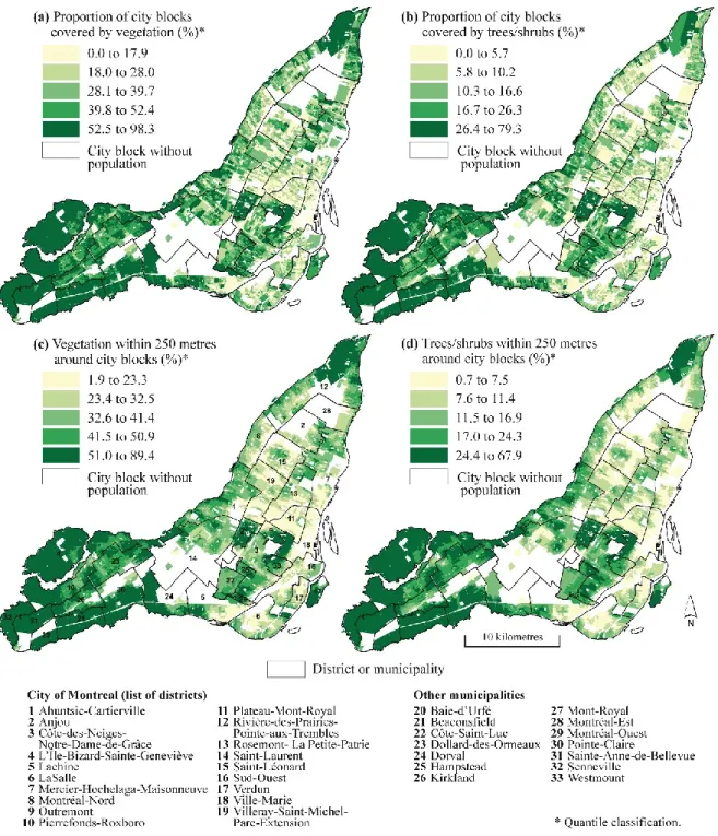
To simplify matters, and also due to lack of space, the vegetation indicators in the block and within 250 metres 200
around the block are only being presented, for a total of four indicators (Figure 1). It should however be noted 201
that the results mapped within 500 metres around the block are very similar to those within 250 metres. 202
Moreover, the indicators are only mapped for blocks on the Island of Montreal with a resident population. It 203
should also be noted that the choropleth maps in Figure 1 are built by using the quantiles classification with five 204
classes (i.e quintiles). That means each category contains 20% of 10210 blocks which makes it possible to easily 205
compare the four maps. 206
Figure 1 shows that the vegetation indicators clearly vary considerably across the Island of Montreal’s territory. 207
For boroughs within the City of Montreal, there is a fairly clear gradient from the centre to the periphery for the 208
four indicators overall: blocks in more densely-populated central boroughs of the Island of Montreal (Ville-209
Marie and Plateau-Mont-Royal) often show less vegetation compared with blocks in more outlying boroughs 210
(Rivière-des-Prairies-Pointe-aux-Trembles, Ahuntsic-Cartierville and Pierrefonds-Roxboro). And it is no 211
surprise that blocks in suburban municipalities at the western end of the island, as well as in wealthier 212
municipalities in the centre of the island (Mont-Royal, Westmount, Côte-Saint-Luc, Hampstead and Montréal-213
Ouest with high median household income and low proportion of low-income households) (Apparicio, Cloutier, 214
& Shearmur, 2007; Séguin, et al., 2012), show higher levels of vegetation. 215
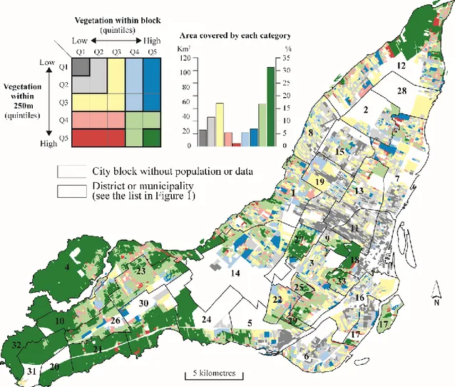
The cross tabulation of the quintiles of two vegetation indicators—the percentages of vegetation in the block and 216
within 250 metres around the block (Figure 1a and 1c)—is mapped in Figure 2. Nine categories of blocks are 217
thus obtained. The two categories in grey are characterized by little vegetation both in the block and within a 218
250-metre radius. Blocks in dark grey (the first quintile for the two indicators) cover 6.5% of the surface area of 219
the Island of Montreal, compared with 11.5% for blocks in light grey. These two types of blocks are mostly 220
found in central boroughs of the City of Montreal: that is, in Ville-Marie, Plateau-Mont-Royal and Mercier-221
Hochelaga-Maisonneuve (Figure 2). At the opposite extreme, the two types of blocks in green consist of blocks 222
in the last quintiles of the two vegetation indicators: that is, those with the highest levels of vegetation in and 223
around the city block. They are very often found in municipalities in the West Island and in wealthy 224
municipalities in the centre of the island such as Mont-Royal and Westmount. Blocks in dark green (the fifth 225
quintile for both indicators) in fact cover 31% of the total surface area of residential blocks, compared with 226
16.6% for blocks in light green. Blocks in red (6.6%) and blue (10.9%) present distinct particularities in terms of 227
vegetation cover. In red are areas with low or medium levels of vegetation within the block (Q1 to Q3), but high 228
levels of vegetation around the block (Q4 and Q5). These are mainly blocks with generally impervious surfaces 229
situated next to a large city park. Areas in blue have high levels of vegetation within the block (Q4 and Q5), but 230
10
low or medium levels of vegetation around the block (Q1 to Q3). These may for example include very green 231
residential blocks typically found in suburbs adjacent to industrial or commercial areas. Finally, blocks in yellow 232
(16.6%) have medium levels of vegetation. 233
234
Figure 1. Vegetation indicators at the city block level
235 236 237
11 238
Figure 2. Typology of city blocks according to the two vegetation indicators
239 240
4.2. Environmental inequity assessment without controlling for the built environment: T-test analysis
241
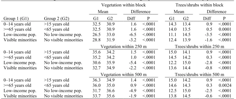
The results of the T-tests presented in Table 2 are used to compare the mean values of the four vegetation 242
indicators when they are weighted by the numbers of each of the groups studied compared with the rest of the 243
population. They clearly show that low-income people live in environments with proportionately less vegetation 244
in and around their residential city block: a difference of -6.5 percentage points for the total vegetation in the 245
block, and of -5.4 and -4.9 percentage points within 250 and 500 metres around the block (p<0.001); and 246
differences of -3.5, -2.8 and -2.5 respectively for the indicators of the percentage of trees in the block, and within 247
250 and 500 metres (p<0.001). The same finding applies for visible minorities, but to a lesser extent, as the 248
differences are smaller: -3.2, -2.2 and -1.9 percentage points respectively for the total vegetation indicators 249
(p<0.001). On the other hand, the situation is more favourable for young people under 15 years old and for 250
seniors aged 65 and over, as they tend to live in environments with more vegetation and more trees in and 251
around their residential city blocks. 252
12
Table 2. Means of vegetation indicators from the T-test for the four groups studied and the rest of the population.
253
Vegetation within block Trees/shrubs within block
Mean Difference Mean Difference
Group 1 (G1) Group 2 (G2) G1 G2 Diff P G1 G2 Diff P
0–14 years old >15 years old 32.5 30.9 1.6 <.0001 14.3 13.4 0.9 <.0001 >=65 years old <65 years old 32.5 30.9 1.6 <.0001 14.0 13.5 0.5 0.0001 Low-income pop. No low-income pop. 26.5 33.0 -6.5 <.0001 11.1 14.5 -3.5 <.0001 Visible minorities No visible minorities 28.8 31.9 -3.2 <.0001 12.4 13.9 -1.6 <.0001
Vegetation within 250 m Trees/shrubs within 250 m
0–14 years old >15 years old 35.6 34.2 1.5 <.0001 15.0 14.1 0.9 <.0001 >=65 years old <65 years old 35.2 34.2 1.0 <.0001 14.5 14.2 0.3 <.0001 Low-income pop. No low-income pop. 30.6 35.9 -5.4 <.0001 12.2 15.0 -2.8 <.0001 Visible minorities No visible minorities 32.7 34.9 -2.2 <.0001 13.6 14.4 -0.8 <.0001
Vegetation within 500 m Trees/shrubs within 500 m
0–14 years old >15 years old 36.3 34.9 1.4 <.0001 15.0 14.2 0.9 <.0001 >=65 years old <65 years old 36.0 35.0 0.9 <.0001 14.6 14.3 0.3 0.0024 Low-income pop. No low-income pop. 31.7 36.6 -4.9 <.0001 12.5 15.0 -2.5 <.0001 Visible minorities No visible minorities 33.7 35.6 -1.9 <.0001 13.8 14.5 -0.6 <.0001
If the variances of the two groups are unequal (with P < 0.05), the Satterthwaite variance estimator is used for the T-test; otherwise, the pooled variance estimator is used.
4.3. Environmental inequity assessment when controlling for the built environment
254
4.3.1. Results of the seemingly unrelated regression models
255
Prior to an analysis of the coefficients of the SUR models, it should be emphasized that the correlations between 256
the residuals of the two equations for models A to D are all highly positive (Table 3). This justifies the use of 257
SUR models (Grene, 2011), as the coefficients of the ordinary least squares (OLS) models would have been 258
biased. It should point out straight away that for all the equations in the four SUR models, the population density 259
and median age of residential buildings have a significant effect on the amount of vegetation. It is not surprising 260
that the logarithm of population density (inhabitants per hectare) is negatively associated with the proportion of 261
vegetation in the block. Furthermore, the relationship between the age of the residential buildings and the 262
vegetation indicators is not linear, but rather curvilinear, which is in keeping with the results of earlier studies 263
(Grove, et al., 2006; Landry & Chakraborty, 2009; Mennis, 2006; Pham, et al., 2013; Pham, et al., 2012). 264
Once the three independent variables of the built environment have been controlled for (population density and 265
median age of residential buildings and its squared form), an examination of the coefficients of the SUR models 266
for the variables of the four groups studied reveals several interesting findings regarding the distributional equity 267
of vegetation in Montreal. 268
In all the SUR models (A to D, Table 3), the coefficients of the percentages of children under 15 years old and of 269
the elderly are positive and significant (p<0.001). The coefficients are in fact much higher for young people than 270
for seniors: for example, in model A, they are 0.979 and 0.330 respectively for equation 1, and 0.797 and 0.173 271
13
for equation 2. This means that, all other things being equal, these two groups are in an advantageous situation in 272
terms of the amount of vegetation and trees in and around the block where they live, especially in the case of 273
children under age 15. The opposite situation is found for the low-income population, with negative and 274
significant coefficients (p<0.001) for all the equations in the four SUR models ranging from -0.285 to -0.327 for 275
models A and B (total vegetation indicators) and from -0.195 to -0.223 for models C and D (trees/shrubs 276
indicators). 277
Table 3. Seemingly unrelated regression models.
278
Model A:
Eq. 1. (DV: vegetation within block) Eq. 2. (DV: vegetation within 250 m)
Model B:
Eq. 1. (DV: vegetation within block) Eq. 2. (DV: vegetation within 500 m)
Equation 1 Equation 2 Equation 1 Equation 2
Coef. T Coef. T Coef. T Coef. T
Intercept 30.689*** 33.82 41.342*** 45.90 30.723*** 33.61 43.621*** 50.65 Inhab./ha (log) -1.824*** -42.18 -3.132*** -24.17 -1.864*** -42.75 -2.902*** -24.47 MedAgeBuild 0.288*** 18.24 0.217*** 11.94 0.308*** 19.03 0.161*** 8.47 MedAgeBuild2 -0.002*** -17.52 -0.002*** -16.37 -0.002*** -18.36 -0.002*** -14.07 0-14 years old (%) 0.979*** 31.78 0.797*** 31.87 0.968*** 31.37 0.717*** 30.28 65 years old and over (%) 0.330*** 18.12 0.173*** 11.59 0.324*** 17.73 0.135*** 9.59 Visible minorities (%) -0.021* -2.14 -0.086*** -10.73 -0.020* -2.05 -0.087*** -11.72 Low-income population (%) -0.325*** -29.37 -0.327*** -36.77 -0.322*** -28.97 -0.285*** -34.08
R2 0.470 0.483 0.471 0.488
Correlation of the residuals 0.597 0.527
AIC for the two models 155,377 155,157
Model C:
Eq. 1. (DV: trees/shrubs within block) Eq. 2. (DV: trees/shrubs within 250 m)
Model D:
Eq. 1. (DV: trees/shrubs within block) Eq. 2. (DV: trees/shrubs within 500 m)
Equation 1 Equation 2 Equation 1 Equation 2
Coef. T Coef. T Coef. T Coef. T
Intercept 7.681*** 13.00 13.010*** 21.79 7.049*** 11.81 13.671*** 23.08 Inhab./ha (log) -0.914*** -32.64 -2.217*** -25.83 -0.937*** -32.99 -2.097*** -25.69 MedAgeBuild 0.274*** 27.81 0.245*** 21.10 0.306*** 29.97 0.208*** 16.40 MedAgeBuild2 -0.002*** -23.00 -0.002*** -19.73 -0.002*** -24.89 -0.002*** -15.79 0-14 years old (%) 0.608*** 30.00 0.571*** 33.92 0.605*** 29.74 0.544*** 33.01 65 years old and over (%) 0.206*** 17.22 0.114*** 11.40 0.203*** 16.83 0.098*** 9.96 Visible minorities (%) 0.013* 1.99 -0.014** -2.59 0.015* 2.35 -0.014** -2.71 Low-income population (%) -0.222*** -30.54 -0.214*** -35.81 -0.223*** -30.58 -0.195*** -33.47
R2 0.400 0.413 0.402 0.399
Correlation of the residuals 0.685 0.610
AIC for the two equations 137,051 138,009
DV: dependent variable.
Signif. codes: *** 0.001, ** 0.01, * 0.05.
For equation 2, the three independent variables relating to the built environment (Inhab./ha (log), MedAgeBuild and MedAgeBuild2)
are calculated within a radius of 250 m or 500 m, excluding the block.
Again, as seen in the T-test analyses, there is less distributional inequity for visible minorities. Indeed, although 279
the coefficients are significantly negative, they are much weaker than for the percentage of low-income 280
individuals for models A and B (varying from -0.020 to -0.087). Moreover, for equation 1 in models A and B, 281
the coefficients are only significant at a threshold of 0.05. Finally, models C and D show that the percentage of 282
14
visible minorities is weakly but positively associated (p=0.05) with the indicator of trees/shrubs within the block, 283
but negatively associated with the same indicator within 250 metres around the block (p<0.01). 284
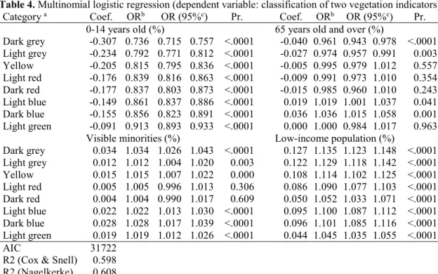
4.3.2. Results of the multinomial logistic regression model
285
The multinomial logistic regression model is built with the dark green category (the greenest blocks both within 286
and around their boundaries) as the reference category (Figure 2). This model is used to determine whether the 287
proportion of each of the four population groups increases the probability that the block belongs to one of the 288
categories in the cross tabulation of vegetation, compared with the dark green category in the tabulation. It 289
should be noted that the odds ratios shown in Table 4 were obtained after controlling for the characteristics of 290
the built environment (population density, median age of residential buildings and its squared form) within the 291
block and within a 250-metre radius of the block, excluding the block itself. However, for purposes of 292
simplification, the coefficients and odds ratios for the variables relating to the built environment are not shown. 293
The results indicate that young people under 15 years old are in a favourable situation, as the odds ratios are all 294
less than 1 and significant (p˂0.0001). This means that, all other things being equal, an increase in the 295
percentage of young people lowers the probability of their block belonging to the dark grey to green categories 296
(blocks that are the least green to blocks that are moderately green both within and around their boundaries) 297
compared with the dark green reference category. The lowest odds ratios are in fact found for categories 298
covering areas with the least vegetation in and around the block (dark grey: 0.736; light grey: 0.792). 299
The situation is more complex for older people, as several of the coefficients are not significant at a threshold of 300
5%. Compared with the greenest blocks, an increase in the percentage of people aged 65 and over decreases the 301
probability of their block being in areas with the least vegetation (dark grey: 0.943; light grey: 0.974), but to a 302
lesser extent than for young people under 15 years of age. Moreover, an increase in the percentage of seniors 303
increases the probability of their block being in areas characterized by a large amount of vegetation within the 304
block but little vegetation within a 250-metre radius (light blue: 1.019; dark blue: 1.036). In sum, people aged 65 305
and over nonetheless enjoy a favourable situation overall. 306
The situation is very different for low-income individuals, as all the odds ratios are greater than 1 and significant 307
(p<0.0001). The highest odds ratios are indeed associated with the least green categories (dark grey: 1.135; light 308
grey: 1.129). Similar results are obtained for people stating that they are members of visible minorities, although
309
their odds ratios, despite being positive, are nevertheless closer to 1 (for example: dark grey: 1.026; light grey: 310
1.012). 311
15
Table 4. Multinomial logistic regression (dependent variable: classification of two vegetation indicators)
313
Category a Coef. ORb OR (95%c) Pr. Coef. ORb OR (95%c) Pr. 0-14 years old (%) 65 years old and over (%)
Dark grey -0.307 0.736 0.715 0.757 <.0001 -0.040 0.961 0.943 0.978 <.0001 Light grey -0.234 0.792 0.771 0.812 <.0001 -0.027 0.974 0.957 0.991 0.003 Yellow -0.205 0.815 0.795 0.836 <.0001 -0.005 0.995 0.979 1.012 0.557 Light red -0.176 0.839 0.816 0.863 <.0001 -0.009 0.991 0.973 1.010 0.354 Dark red -0.177 0.837 0.803 0.873 <.0001 -0.015 0.985 0.960 1.010 0.243 Light blue -0.149 0.861 0.837 0.886 <.0001 0.019 1.019 1.001 1.037 0.041 Dark blue -0.155 0.856 0.823 0.891 <.0001 0.036 1.036 1.015 1.058 0.001 Light green -0.091 0.913 0.893 0.933 <.0001 0.000 1.000 0.984 1.017 0.963
Visible minorities (%) Low-income population (%)
Dark grey 0.034 1.034 1.026 1.043 <.0001 0.127 1.135 1.123 1.148 <.0001 Light grey 0.012 1.012 1.004 1.020 0.003 0.122 1.129 1.118 1.142 <.0001 Yellow 0.015 1.015 1.007 1.022 0.000 0.108 1.114 1.102 1.125 <.0001 Light red 0.005 1.005 0.996 1.013 0.306 0.086 1.090 1.077 1.103 <.0001 Dark red 0.004 1.004 0.990 1.017 0.609 0.050 1.052 1.033 1.071 <.0001 Light blue 0.022 1.022 1.013 1.030 <.0001 0.095 1.100 1.087 1.112 <.0001 Dark blue 0.028 1.028 1.017 1.039 <.0001 0.096 1.101 1.085 1.116 <.0001 Light green 0.019 1.019 1.012 1.026 <.0001 0.044 1.045 1.035 1.055 <.0001 AIC 31722
R2 (Cox & Snell) 0.598 R2 (Nagelkerke) 0.608
a See the categories in Figure 2. Reference category: Dark green. b Odds ratio. c 95% Wald confidence limits.
The reported values were obtained after controlling for population density (logarithm of inhabitants/ha), median age of residential buildings and squared median age of residential buildings.
314
5. Discussion and conclusion
315
The different types of analyses used in this study show that in Montreal, children and, to a lesser degree, older 316
people enjoy quite an advantageous situation: they more often live in areas with high levels of vegetation in and 317
around their city blocks. Environmental inequities, on the other hand, are more strongly associated with people’s 318
income levels than with their belonging to an ethnocultural or racial group, which corroborates the findings of 319
several earlier studies on urban vegetation in Baltimore (Troy, et al., 2007), Tampa (Landry & Chakraborty, 320
2009), Vancouver and Toronto (Tooke, et al., 2010). The use of vegetation indicators in and around the block 321
makes it possible to demonstrate the existence of a double inequity in some areas of the city for these two 322
groups, which previous studies had not shown. A double inequity of this kind is worrisome, given the negative 323
impacts of a lack of vegetation on the public health of these populations. 324
This double inequity in terms of access to vegetation can in fact affect different population groups differently, 325
depending on their level of income. Well-off households living in an area with little greenery—in a downtown 326
residential tower, for example—can more easily remedy the lack of vegetation: with air conditioning, by staying 327
at their secondary residence in the country on weekends or while on vacation, etc. Low-income households, on 328
the other hand, tend to be more confined to their neighbourhoods all year long, as they often have less access to a 329
motor vehicle. The lack of vegetation in neighbourhoods with high residential densities contributes to the heat 330
16
island effect during the heat waves that sometimes strike Montreal in the summer, which can have disastrous 331
consequences for some population groups, particularly the elderly (Smargiassi, et al., 2009). So, because all 332
citizens are not equally able to cope with a lack of vegetation, it might be better to think in terms, not of 333
distributional equity, but rather of compensatory equity (Apparicio & Séguin, 2006; Talen, 1998) in order to 334
ensure that disadvantaged neighbourhoods have their fair share of vegetation. 335
Several possible reasons can be advanced to explain the higher proportion of low-income households in 336
vegetation-deprived areas. For example, it may be due to the lower cost of both rental housing and home 337
ownership in areas with less vegetation (Donovan & Butry, 2010). Also, Heynen (2006) mentions that 338
households with limited financial means tend to place less emphasis, for various reasons, on the importance of 339
vegetation. In regard to disparities affecting visible minorities, it is possible that they are being discriminated 340
against in terms of their access to green living environments. 341
The approach developed here, which combines multisource data and remote sensing, GIS and spatial analysis 342
methods, would seem to be an especially interesting technique for planning urban greening interventions. 343
Mapping the different types of blocks according to the level of abundance of vegetation—both in and around 344
these blocks—(in the cross tabulation of two vegetation indicators) could represent a very useful tool for urban 345
planners. It can in fact be used to target areas that could benefit from greening campaigns. Nonetheless, Wolch, 346
Byrne, and Newell (2014, p. 235) note that greening projects in disadvantaged neighbourhoods “can, however, 347
create an urban green space paradox” by making these areas also more attractive to wealthier households, thus 348
contributing to their gentrification and prompting disadvantaged households to leave the area. Greening projects 349
should therefore be implemented on a local scale and involve the communities living in these neighbourhoods. 350
In this sense, the results of this paper could help urban planners to design greening interventions. For example, in 351
vegetation-deprived areas within the block, measures to foster the greening of private gardens, urban agriculture, 352
or green walls and roofs are some of the initiatives that could be emphasized. In vegetation-deprived areas 353
around the block, priority could be given to planting trees along the streets or to developing a new urban park. 354
Interventions of this kind would help to reduce the environmental inequities that low-income people and visible 355
minorities face. 356
Acknowledgments
357
The authors would like to thank the anonymous reviewers for their careful reading of our manuscript and their 358
many insightful comments and suggestions. The authors also wish to thank the Canada Research Chair in 359
Environmental Equity and the City (SSHRC) for their financial support. 360
17
References
361
Apparicio, P., Abdelmajid, M., Riva, M., & Shearmur, R. (2008). Comparing alternative approaches to measuring the 362
geographical accessibility of urban health services: Distance types and aggregation-error issues. International Journal of 363
Health Geographics, 7 (7), 1-14. 364
Apparicio, P., Cloutier, M.-S., & Shearmur, R. (2007). The case of Montreal's missing food deserts: evaluation of 365
accessibility to food supermarkets. International Journal of Health Geographics, 6 (1), 1-13. 366
Apparicio, P., & Séguin, A.-M. (2006). Measuring the accessibility of services and facilities for residents of public housing 367
in Montréal. Urban Studies, 43 (1), 187-211. 368
Apparicio, P., Séguin, A.-M., & Naud, D. (2008). The quality of the urban environment around public housing buildings in 369
Montréal: An objective approach based on GIS and multivariate statistical analysis. Social Indicators Research, 86 (3), 370
355-380. 371
Bowen, W. (2002). An analytical review of environmental justice research: what do we really know? Environmental 372
management, 29 (1), 3-15. 373
Briggs, D., Abellan, J. J., & Fecht, D. (2008). Environmental inequity in England: small area associations between socio-374
economic status and environmental pollution. Social Science & Medicine, 67 (10), 1612-1629. 375
Carrier, M., Apparicio, P., Kestens, Y., Séguin, A.-M., Pham, H., Crouse, D., & Siemiatycki, J. (2016). Application of a 376
Global Environmental Equity Index in Montreal: Diagnostic and Further Implications. Annals of the American Association 377
of Geographers, 1-18. 378
Carrier, M., Apparicio, P., Séguin, A.-M., & Crouse, D. (2014a). Ambient air pollution concentration in Montreal and 379
environmental equity: Are children at risk at school? Case Studies on Transport Policy, 2 (2), 61-69. 380
Carrier, M., Apparicio, P., Séguin, A.-M., & Crouse, D. (2014b). The application of three methods to measure the statistical 381
association between different social groups and the concentration of air pollutants in Montreal: A case of environmental 382
equity. Transportation Research Part D: Transport and Environment, 30, 38-52. 383
City of Montréal. (2011). Plan d'action canopée 2012-2021. In Direction des grands parcs et du verdissement (pp. 12). 384
City of Toronto. (2013). Sustaining & expanding the urban forest: Toronto’s strategic forest management plan. In Parks, 385
Forestry and Recreation Division (pp. 83). 386
Cutter, S. L., Holm, D., & Clark, L. (1996). The role of geographic scale in monitoring environmental justice. Risk Analysis, 387
16 (4), 517-526. 388
de Vries, S., van Dillen, S. M., Groenewegen, P. P., & Spreeuwenberg, P. (2013). Streetscape greenery and health: Stress, 389
social cohesion and physical activity as mediators. Social Science & Medicine, 94, 26-33. 390
Donovan, G. H., & Butry, D. T. (2010). Trees in the city: Valuing street trees in Portland, Oregon. Landscape and Urban 391
Planning, 94 (2), 77-83. 392
Grene, W. H. (2011). Econometric Analysis (7th edition). Econometric analysis, Upper Saddle River, NJ. 393
Grove, J. M., Cadenasso, M. L., Burch, W. R., Pickett, S. T. A., Schwarz, K., O'Neil-Dunne, J., Wilson, M., Troy, A., & 394
Boone, C. (2006). Data and methods comparing social structure and vegetation structure of urban neighborhoods in 395
Baltimore, Maryland. Society and Natural Resources, 19, 117-136. 396
Henningsen, A., & Hamann, J. A. (2015). Systemfit: A package for estimating systems of simultaneous equations in R. In, 397
R package version 1.1-18. 398
Heynen, N. (2006). Green urban political ecologies: toward a better understanding of inner-city environmental change. 399
Environment and Planning A, 38, 499-516. 400
Hubacek, K., & Kronenberg, J. (2013). Synthesizing different perspectives on the value of urban ecosystem services. 401
Landscape and Urban Planning, 1 (109), 1-6. 402
Landry, S. M., & Chakraborty, J. (2009). Street trees and equity: evaluation the spatial distribution of an urban amenity. 403
Environment and Planning A, 41, 2651-2670. 404
Landry, S. M., & Pu, R. (2010). The impact of land development regulation on residential tree cover: An empirical 405
evaluation using high-resolution IKONOS imagery. Landscape and Urban Planning, 94 (2), 94-104. 406
Mennis, J. (2006). Socioeconomic-vegetation relationships in urban, residential land: The case of Denver, Colorado. 407
Photogrammetric Engineering & Remote Sensing, 72 (8), 911-921. 408
Mullaney, J., Lucke, T., & Trueman, S. J. (2015). A review of benefits and challenges in growing street trees in paved urban 409
environments. Landscape and Urban Planning, 134, 157-166. 410
Pham, T.-T.-H., Apparicio, P., Landry, S. M., Séguin, A.-M., & Gagnon, M. (2013). Predictors of the distribution of street 411
and backyard vegetation in Montreal, Canada. Urban Forestry and Urban Greening, 12 (1), 18-27. 412
Pham, T.-T.-H., Apparicio, P., Séguin, A.-M., & Gagnon, M. (2011). Mapping the greenscape and environmental equity in 413
Montreal: An application of remote sensing and GIS. In S. Caquard, L. Vaughan & W. E. Cartwright (Eds.), Mapping 414
Environmental Issues in the City. Arts and Cartography Cross Perspectives (pp. 30-48). Springer. 415
18
Pham, T.-T.-H., Apparicio, P., Séguin, A.-M., Landry, S. M., & Gagnon, M. (2012). Spatial distribution of vegetation in 416
Montreal: An uneven distribution or environmental inequity? Landscape and Urban Planning, 107 (3), 214-224. 417
Roy, S., Byrne, J., & Pickering, C. (2012). A systematic quantitative review of urban tree benefits, costs, and assessment 418
methods across cities in different climatic zones. Urban Forestry & Urban Greening, 11 (4), 351-363. 419
Schwarz, K., Fragkias, M., Boone, C. G., Zhou, W., McHale, M., Grove, J. M., O’Neil-Dunne, J., McFadden, J. P., 420
Buckley, G. L., & Childers, D. (2015). Trees grow on money: urban tree canopy cover and environmental justice. PloS 421
one, 10 (4), 1-17. 422
Séguin, A.-M., Apparicio, P., & Riva, M. (2012). Identifying, mapping and modelling trajectories of poverty at the 423
neighbourhood level: the case of Montréal, 1986–2006. Applied Geography, 35 (1), 265-274. 424
Séguin, A.-M., Apparicio, P., & Riva, M. (2015). The changing spatial distribution of Montreal seniors at the 425
neighbourhood level: a trajectory analysis. Housing Studies. 426
Smargiassi, A., Goldberg, M. S., Plante, C., Fournier, M., Baudouin, Y., & Kosatsky, T. (2009). Variation of daily warm 427
season mortality as a function of micro-urban heat islands. Journal of Epidemiology and Community Health, 63 (8), 659-428
664. 429
Talen, E. (1998). Visualizing fairness: Equity maps for planners. Journal of the American Planning Association, 64 (1), 22-430
38. 431
Taylor, M. S., Wheeler, B. W., White, M. P., Economou, T., & Osborne, N. J. (2015). Research note: Urban street tree 432
density and antidepressant prescription rates—A cross-sectional study in London, UK. Landscape and Urban Planning, 433
136, 174-179. 434
Tooke, T. R., Klinkenberg, B., & Coops, N. C. (2010). A geographical approach to identifying vegetation-related 435
environmental equity in Canadian cities. Environment and Planning B: Planning and Design, 37, 1040-1056. 436
Troy, A. R., Grove, J. M., O'Neil-Dunne, J. P. M., Pickett, S. T. A., & Cadenasso, M. L. (2007). Predicting opportunities for 437
greening and patterns of vegetation on private urban lands. Environ Manage, 40, 394-412. 438
Walker, G. (2012). Environmental Justice: Concepts, Evidence and Politics. Routledge, New York. 439
Wolch, J. R., Byrne, J., & Newell, J. P. (2014). Urban green space, public health, and environmental justice: The challenge 440
of making cities ‘just green enough’. Landscape and Urban Planning, 125, 234-244. 441
Zellner, A. (1962). An efficient method of estimating seemingly unrelated regressions and tests for aggregation bias. 442
Journal of the American statistical Association, 57 (298), 348-368. 443
Zellner, A. (1963). Estimators for seemingly unrelated regression equations: Some exact finite sample results. Journal of the 444
American statistical Association, 58 (304), 977-992. 445
446 447