To link to this article:
DOI:10.1016/j.engappai.2018.04.001
URL:
https://doi.org/10.1016/j.engappai.2018.04.001
This is an author-deposited version published in: http://oatao.univ-toulouse.fr/
Eprints ID: 19945
To cite this version
:
Lachhab, Majda and Béler, Cédrick and Coudert, Thierry A risk-based
approach applied to system engineering projects: a new learning based
multi-criteria decision support tool based on an ant colony algorithm.
(2018) Engineering Applications of Artificial Intelligence, vol. 72. pp.
310-326. ISSN 0952-1976
O
pen
A
rchive
T
oulouse
A
rchive
O
uverte (
OATAO
)
OATAO is an open access repository that collects the work of Toulouse researchers and
makes it freely available over the web where possible.
Any correspondence concerning this service should be sent to the repository
administrator:
[email protected]
A risk-based approach applied to system engineering projects: A new
learning based multi-criteria decision support tool based on an Ant Colony
Algorithm
Majda Lachhab
*
, Cédrik Béler, Thierry Coudert
INP-ENIT/LGP, University of Toulouse, 47 Avenue d’Azereix, 65000 Tarbes, France
Keywords: Project management System engineering Uncertainty Risk MONACO Decision support Learning
A B S T R A C T
This article proposes a multi-criteria decision support tool fully integrated within system engineering and project management processes that allows decision makers to select an optimal scenario of a project. A model based on an oriented graph includes all the alternative choices of a new system’s conception and realization. These choices take into account the risks inherent to perform project tasks in terms of cost and duration. The model of the graph is constructed by considering all the collaborative decisions of the different actors involved in the project. This decision support tool is based on an Ant Colony Algorithm (ACO) for its ability to provide optimal solutions in a reasonable amount of time. The model developed is a multi-objective new ant colony algorithm based on an innovative learning mechanism (named MONACO) that allows ants to learn from their previous choices in order to influence the future ones. The objectives to be minimized are the total cost of the project, its global duration and the risk associated with these criteria. The risk is modeled as an uncertainty related to the increase of the nominal values of cost and duration. The optimization tool is a part of an integrated and more global process, based on industrial standards (the System Engineering process and the Project Management one) that are widely known and used in companies.
1. Introduction
Whenever complexity exists, risks exist too. The difficulty to make concerted decisions between all the actors of a Project Management (PM) process and a System Engineering (SE) one increases the complex-ity of a SE project. For this purpose, an integrated process that takes into account the interactions between the PM and the SE sub-processes is a good way to make collaborative decisions and meet the customer needs by satisfying the different requirements and project objectives especially in terms of cost, duration and risk. Some previous works done in our research team have defined coupling points between a system design process and a project planning process (Coudert et al., 2011;
Vareilles et al., 2015). These works have shown that both processes need to be controlled and executed in parallel with strong synchronization mechanisms which allow meeting the requirements of the customers. A centralized information model (represented by an oriented graph) is useful to consider all the decisions of these project actors about all the possible tasks and their associated project objectives values. Making good decisions among all these possible choices needs to select the optimized ones. In our work, the objectives to optimize are the global
* Corresponding author.
E-mail addresses:[email protected](M. Lachhab),[email protected](C. Beler),[email protected](T. Coudert).
cost of the project, its total duration and the global risk associated to these criteria. Risks are defined in this work as uncertainty about project objectives and are considered in the preliminary steps of a project graph construction. Uncertainty is modeled by using intervals to take into account the negative risks’ impacts on tasks costs and durations. The idea is to provide to the decision makers a panel of Pareto-optimal solutions in order to select one good scenario to plan and then realize.
The proposed integrated process includes a multi-criteria decision support tool based on a multi-objective optimization method. It allows the generation of Pareto-optimal scenarios from the resulting integrated project graph that encompasses all the design and the project alternative choices of a new system to conceive and realize. For this matter,
the standard Ant Colony Optimization (ACO) meta-heuristic (Dorigo
and Stützle, 2010; Stützle et al., 2011) was adopted and adapted to develop a multi-objective new ant colony algorithm based on a learning mechanism denoted as MONACO algorithm.
The standard ACO algorithm performance is improved by a learning mechanism. That consists in modifying the standard probability formula used by every ant to reach a next node in the graph. It is modified taking
into account the path that every ant has taken before the decision. The proposed learning mechanism learns from the past choices made by an ant in order to influence its future ones by changing dynamically the weights given to the three objectives (cost, duration, risk) in the probability formula of the MONACO algorithm. At the end of the algorithm, a Pareto-front is built and all the optimal scenarios are given to help the decision makers to select one scenario that has reasonable global values of cost, duration and risk.
A related works section is given in the next part (Section 2) to contextualize the problematic with regards to other works and to justify the use of an Ant Colony Algorithm. Then, a detailed description of the integrated SE and PM process is presented in Section3with the different project actors that may be involved in all the project phases. The problem formalization is described in the same section. The proposed multi-criteria decision support tool based on the MONACO algorithm
is detailed in Section 4. The algorithm is developed by using Ruby
language and some experiments have been conducted and presented in the results section (cf. Section5). Finally, conclusions and future works are described in Section6.
2. Related works
The design and the generation of new systems are industrial activities that are complex to manage in a very competitive market. In this context, system engineers and project managers need an efficient risk management process to face the various technical and programmatic risks that may arise during the project (SEBOK Guide, 2014). Previous works have defined the interactions between systems design and project planning processes to better control them. In Abeille et al. (2010) andCoudert et al.(2011), structural interactions to establish bijective connections between system and project structures have been defined. Another model of behavioral interaction has been proposed inVareilles et al. (2015) allowing synchronization of system design and project planning by defining the rules that are related to a specific integrated
model. The risk management process (PMBOK Guide, 2013) is not
carried out during the early phases of the project elaboration. It is rather done during the project activity planning process to estimate the tasks costs and durations, as well as all resources related to design, production and distribution activities. That is why we propose an integrated process where risks are taken into account upstream.
Risk exists whenever there is uncertainty (Better and Glover, 2008). Many works in the literature provide the fundamental principles on how to manage, characterize and assess risk by giving the appropriate concepts and management tools to support the decision making in
practice (Aven, 2016). Thus, many risk management methods use
qualitative and quantitative approaches to assess the risk with some
tools that are based on the probability and impact concepts (Fang
and Marle, 2012). Recent directions of development to represent un-certainty in risk assessment are provided in Flage et al. (2014). In this article, many methods are used to handle the uncertainty but the predominant one is the probabilistic analysis method to handle both random and epistemic uncertainty. InAqlan and Ali(2014), the uncertainty inherent in risks is performed by using lean principles and fuzzy bow-tie analysis to improve the risk management process in the chemical industry. InVilleneuve et al.(2016), the authors proposed to improve the risk assessment by using the theory of belief functions and statistical knowledge combined with the expert knowledge for aircraft deconstruction. In the case of supplier selection problem, the
authors in Kaya and Karhaman(2010) developed a decision making
tool that evaluates risks by using fuzzy logic models. In Ward and
Chapman(2003), the authors considered the risk management processes as projects uncertainty management processes. For large engineering projects, a network theory based approach was presented inFang et al.
(2012) to deal with the interdependencies between negative risks and to better understand their potential interactions by using network theory indicators in project risk analysis. InNguyen et al.(2013), the ProRisk
methodology has been developed to provide to project managers a decision making tool to select the best risk treatment strategy. In the same context, inFan et al. (2008) an analytical model based on a conceptual framework that describes the quantitative relationships between risk-handling strategy and the various project characteristics (technical complexity, project size, slack) has been proposed. Some
works are based on an improved CPM (Critical Path Method—see
Gal-loway(2006) for instance) because the durations values can be changed considering the multiple risk factors, such as, the use of Monte Carlo Simulation (MCS). However, MCS provides a project risk analysis on project objectives without considering the interdependencies between the different risk factors (Jun-Yan, 2012) which is not in accordance with real-life projects. Bayesian networks (Pearl, 1995) are appropriate to deal with the relationships between the risk factors. For example, inKhodakarami et al. (2007), uncertainty in project scheduling was modeled by means of Bayesian networks considering that the traditional inputs for each activity (cost, time, resources) are not deterministic.
In our approach, uncertainty is defined as the impact of undesirable events on project objectives (cost and duration). It must be considered while making decisions about the structure of the system and its asso-ciated project. The need to optimize each technical choice jointly with those related to project activities has been highlighted in previous works (Pitiot et al., 2010) where a multi-criteria optimization method based on an evolutionary algorithm guided by knowledge has been proposed. The method principle was to optimize the selection of project scenarios, taking into account design choices and project activities associated with them. A scenario is a set of tasks, with precedence constraints, that must be planned. The aim was to obtain a set of Pareto-optimal scenarios in a two-dimensional objective space (the total cost and the overall duration of the project). However, uncertainty was not taken into account. Thus, in order to improve it, a third dimension can be integrated: the risk one. In previous works done in our research team (Baroso et al., 2014), the integration of risk as a third objective to minimize was proposed using a multi-objective algorithm based on a standard ACO. The ACO meta-heuristic is selected for addressing the problem that this paper is dealing with because many works in the literature attest that the use of ACO is very promising in project management especially in providing near optimal solutions to handle issues that are too expensive computationally. InFernandez et al.(2015), the authors have developed a hybrid approach based mainly on ACO meta-heuristic to handle many objectives in the case of portfolio problems. It provided high-quality portfolios compared with other powerful meta-heuristics that deal with Pareto-front solutions. Other works have proved the power of ACO algorithms for solving both deterministic and probabilistic networks such as CPM/PERT by providing good optimal and sub-optimal solutions (Abdallah et al., 2009). InChen and Zhang(2012), the authors used an Ant Colony System (ACS) approach and Monte Carlo simulation (MCS) to maximize under uncertainty the expected net present value (NPV) of cash flows in the case of scheduling multi-mode projects.
Another application of ACO and MCS technique was exploited inAghaie
and Mokhtari (2009) for stochastic project crashing problem under uncertainty. This method has shown the high performance of ACO approach especially on high scale networks.
Moreover, by building the solutions step-by-step within ACO algo-rithms, it is possible to design useful heuristics to direct the ants to avoid critical tasks as early as possible (Chen and Zhang, 2013). This characteristic is a key concept in our work. The improvement of the standard ACO for optimization consists in allowing the ants not only to learn from the previous paths taken by the other ants, but also by guiding each ant in its process of selecting the next node (task) in a project graph. This process is based on a new learning mechanism that considers the path of each ant to influence its next choice by favoring one criterion over another based on the capital consumed in terms of cost, duration and risk. This learning process is reflected in this article through the use of dynamic weights in the probability formula. Therefore, the choice of the ACO meta-heuristic is also driven by these
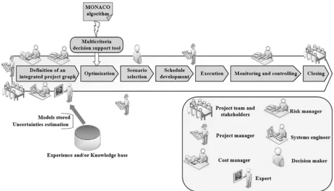
Fig. 1. General framework of the integrated process.
principles. It is necessary to use a method which builds the solutions by searching paths in the project graph node after node. For these reasons, the standard meta-heuristic Ant Colony Optimization has been chosen in order to be improved by our new learning algorithm.
To sum up, the problem this paper is dealing with consists in defining an efficient multi-criteria decision support tool based on a multi-objective optimization model (cost, duration, risk). This tool is integrated into the standard industrial processes (the system engineering
process (SEBOK Guide, 2014) and the project management process
(PMBOK Guide, 2013)) in the early phases of a system engineering project. The adaptation of these standards into one integrated process allows to guarantee that the proposed method will be used efficiently in companies. In this context, the contribution this article is dealing with consists in defining an integrated process wherein the structures of the system and its associated project as well as the risks inherent to this project are jointly constructed, at the earliest, by using ad hoc mechanisms and tools. Thus, the integrated process is supported by means of a multi-criteria decision support tool based on the MONACO algorithm to help the decision makers to select one Pareto-optimal scenario from a project graph that handles all the common decisions of the different project actors and stakeholders. The scenario is a solution that will be planned and executed in the posterior phases of the project. The integrated process is described in the next section.
3. Proposed integrated process
The work carried out in this part consists in defining a global approach where the processes of system engineering and project man-agement (including the processes of cost and risk manman-agement) are articulated efficiently (cf. Section3.1). First ideas were presented in (Lachhab et al., 2017). Our proposed decision support tool must be integrated to allow all the project actors to work on a common (ideally collaborative) model that will enable them to refine the contextual definitions and then the scenarios selection in a project graph. This graph includes all the possible options of design and realization of a new complex system. The decision making, conducted by the different actors,
is assisted by this tool which seeks to minimize the project objectives in terms of cost, duration and risk (cf. Section3.2).
The specificity of our problem, relatively to the traditional ap-proaches of multi-criteria decision support, is the consideration of risk. The difficulty lies in the fact that the risk is not as tangible as the standard criteria of cost and duration but also that the risk has potentially an impact on these two criteria. In this work, this notion of risk is integrated locally as an uncertainty about the objectives of the project (cost, duration) but also globally as a third objective to optimize (cf. Section3.3). In addition, the system engineering and the project management processes are fed by an experience base and/or a knowledge base to control the uncertainty about costs and durations. The multi-criteria decision support tool enables the generation of a panel of Pareto-optimal scenarios (solutions). From this panel, a scenario is selected to be planned and then realized under the control of the project manager.
To perform the decision making process, it was decided to use a specific multi-objective ant colony algorithm (that will be detailed in Section4) for its ability to solve such a combinatorial optimization problem within a reasonable time. The first results were presented in
Lachhab et al.(2016) where a simple instance of the problem was tested without any kind of framework to implement the tool. Thus, the aim of this section is to propose a global framework of integrated industrial processes where the optimization tool is used. This global and general framework is described in the next sections.
3.1. Proposed general framework
Many actors and processes are involved in the realization of a new project. It is proposed then to bring together all the processes of system engineering and project management in a global process that includes our multi-criteria decision support tool (cf. Section 3.3). This tool involves all the project actors for the scenarios selection in a complex project graph. The proposed general methodology is illustrated inFig. 1, where all the sub-processes of the project management (including time, risk and cost management) and system engineering processes are federated into one integrated process.
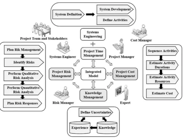
Fig. 2. Definition of an integrated project graph sub-process.
Fig. 3. The optimization framework.
This process includes 7 sub-process groups describing the different phases of a system engineering project. These sub-processes are: defi-nition of an integrated project graph, optimization, scenario selection, schedule development, execution, monitoring and controlling, and fi-nally, closing. A macroscopic view of the system engineering and project management processes integration is shown inFig. 1. All the technical choices of the system and the associated project activities are considered at the earliest phases of the project by all the actors. All these actors collaborate around a common centralized model resulting from their collaborative decisions that are also based on the knowledge capitalized in a knowledge base. This knowledge base includes all the standards, rules, information on uncertainty and some examples of project models. Indeed, the new system to conceive may include some parts that can be specified from similar previous projects or can be designed from scratch. An experience base can also be solicited by an expert to enrich the
resulting information project model. However, it is important to notice that the capitalization and reuse of knowledge and experiences are not described in this article.
Once all the scenarios of the project are built, an optimization process enables to optimize the selection of the project scenarios by using a specific multi-criteria decision support tool based on a new multi-objective ant colony algorithm (cf. Section4).
The optimization seeks to minimize three objectives: cost, duration and risk. Optimizing the risk in this work goes to minimize the un-certainty about the values of cost and duration. The modeling of this uncertainty using intervals is discussed in more detail in Section3.3. Pareto-optimal scenarios within a reasonable time are generated. Thus, only one scenario is then selected by the decision maker to plan it and proceed afterwards to its realization. Once the project scenario is realized, the monitoring process allows the control and the monitoring
of the project performance. The collected information and the lessons learned in the execution phase (realization) are then capitalized in an experience base when closing the project. This experience base can be solicited by an expert to formalize lessons learned and capitalize them in a knowledge base for future use in new projects.
3.2. Detailed sub-processes description 3.2.1. Definition of an integrated project graph
The definition of an integrated project graph sub-process allows the construction of the resulting project model from PM and SE processes integration. The project model is built according to the collaborative decisions made by the project manager, the cost manager, the risk manager, the project team, the stakeholders and the system engineer. An important point is to take into account risks during this step. Many decisions are made in the early phases of the SE project to anticipate and to mitigate the impact of them on the project objectives (cost, duration) during the execution step. The project tasks estimations are the result of discussions made between all the project actors but also according to expert opinions. The definition of an integrated project graph sub-process is in fact the sub-process that enables the construction of the project
model as represented onFig. 2. This figure includes all the project actors
and the sub-processes involved to build the graph. These sub-processes belong to five industrial processes, namely, the system engineering process (System Definition and System Development sub-processes), the project time management process (Define Activities sub-process), the project cost management process (Sequence Activities, Estimate Activity Durations, Estimate Activity Resources and Estimate Cost sub-processes), the project risk management process (Plan Risk Management, Identify Risks, Perform Qualitative Risk Analysis, Perform Quantitative Risk Analysis and Plan Risk Responses sub-processes), and finally, the knowledge
management process (Define Uncertainties sub-process). Thus, Fig. 2
gives a detailed view about the different tasks that are performed by all the project actors within the sub-processes aforementioned.
In the System Definition sub-process, the system engineer contributes in the definition of all the technical requirements by considering the systems safety and reliability, its performances and also the expected systems functional characteristics.
In the System Development sub-process, the system engineer analyses the requirements in order to define the logical and physical structures of the new system to deliver in conjunction with the project manager who defines their associated project activities (Vareilles et al., 2015).
The characteristics associated with each project activity such as the activity name, its predecessors and successors (the logical relationships to sequence activities), the resources required to perform the activities (equipment, materials, competencies and services) and the estimated values of the criteria (cost, duration, risk) are defined. Some preventive activities can be added by the risk manager while defining the project activities to prevent, at the earliest, the risks associated with them.
The activities durations can be estimated by the project manager from historical information using some data-mining tools and tech-niques (Ramageri and Bharati, 2010) or collaboratively with an expert. The activities costs can be estimated by the cost manager by defining the costs of the resources required to perform each activity. An expert can also be solicited to estimate the activities costs from analogous previous projects.
Once the project tasks are defined with their different estimated costs, durations, resources and all the potential risks that may arise during the project realization, a qualitative risk analysis is performed by classifying the risks according to their probabilities of occurrence and their impacts on the project goals (cost, duration). In our work, the quantitative risk analysis sub-process is performed by considering that the risk value is seen as an uncertainty about cost and duration values. This uncertainty is modeled by using intervals where the lower bounds correspond to the nominal values of activities costs and durations and the upper bounds represent their estimated maximum values if undesir-able events occur. The estimations of the nominal project activities costs
and durations values and the uncertainty is obtained from an expert and by analyzing the project past experiences (Béler and Desforges, 2007). The risk response actions are defined in the Plan Risk Responses sub-process. They represent the corrective solutions that are translated in our model by the increase values of costs/durations and are computed by means of a risk indicator. That will contribute in mitigating the impacts of the identified risks in the first phase of the project risk management process.
3.2.2. Optimization sub-process
The multi-criteria decision support tool based on the MONACO algorithm is developed and then used in the optimization sub-process. It aims at minimizing simultaneously the global cost, duration and risk values of the project associated with the project graph. In our model, risk is considered as a third dimension to optimize and represents an uncertainty about the project objectives (cost, duration). The optimiza-tion framework is represented onFig. 3. A file containing the integrated model (i.e. the integrated project graph obtained collaboratively at the previous step) is provided to the MONACO algorithm. From the generated Pareto front, one solution is selected for scheduling and realization.
3.2.3. Scenario selection, schedule development and execution sub-processes Once the Pareto-optimal project scenarios are generated at the end of the MONACO algorithm, a Pareto-front is built. The optimization tool aims to generate solutions which do not favor one objective over another. Thus, the decision maker has the free choice to select one scenario, from the Pareto-front, that gives a trade-off between the global values of the three criteria of the triplet (𝐶, 𝐷, 𝑅). The selected scenario, in the scenario selection sub-process, is scheduled (using a standard scheduling tools) and then executed by the project manager in the schedule development and execution sub-processes.
3.2.4. Monitoring and controlling sub-process
The supervision of executed activities is performed in the monitoring and controlling phase where some corrective response actions are defined and the measurement of project performance is conducted. In fact, the risk manager makes a project control under uncertainty by comparing the real results of the project with the estimated ones to identify the eventual deviations. Some Key Performance Indicators (KPI) are then computed to help the project manager to make decisions consid-ering uncertainty on activities costs and durations (Acebes et al., 2013). 3.2.5. Closing sub-process
At the end of the project realization, experiences are capitalized in an experience base for a future reuse in similar projects. Thus, in our work, the closing sub-process is assimilated to an experience
feedback (EF) process (Béler and Desforges, 2007;Kamsu Foguem et
al., 2008). Current experiences are capitalized into an experience base. From experiences, knowledge is generated and stored in a knowledge base. In our work, the knowledge base includes all the information about uncertainty on specific activities costs and durations that were performed in several previous analogous complex projects.
3.3. Problem formalization
The integrated process defined in Section3.1is based on the use of a generic and integrated project model that contains all the possible scenarios (Fig. 4).
The global model exposed to the different actors is formulated by means of an oriented and acyclic project graph. This graph, denoted by 𝐺 = (𝑁 , 𝐴), which represents a formal representation of our problem, is defined by means of a set of nodes 𝑁 and a set of arcs 𝐴. The arcs connect these nodes and represent the precedence constraints between them. The nodes of the graph represent the project tasks and the conjunction logical operators (AND, AND). The first and the last nodes of the graph
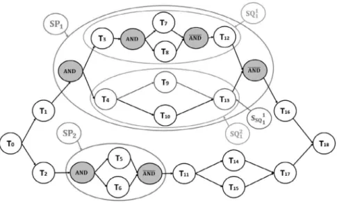
Fig. 4. Example of an integrated project graph.
are fictive (they represent only the beginning and the end of the project). Each task node is associated with a triplet (𝐶, 𝐷, 𝑅) corresponding to the task cost, its duration and the risk values corresponding to these criteria. In this paper, the risk is considered as an uncertainty about the realization of the project tasks. This uncertainty is defined as the occurrence of undesirable events whose impacts increase the total cost of the project and/or its total duration. This uncertainty is modeled by intervals. The lower bound of the interval represents the nominal value of each criterion (cost, duration) and the upper bound corresponds to the maximum value obtained from an expert knowledge and/or from past experiences.
The considered project graph 𝐺 may involve other sub-graphs according to the complexity of the project and its associated project graph. The sub-graph is defined as a sub-project where the starting node is a divergence node (AND) and the ending node is a convergence one (AND). In the example ofFig. 4, SP1and SP2are sub-projects. In
our work, a sub-project is considered as a project or a ‘‘macro-task’’ characterized by its triplet (𝐶, 𝐷, 𝑅). After the first node of the graph, all the technical choices and their corresponding project choices for the new system to design are represented.
The project 𝑃 is formulated, in Eq.(1), as a union of the set of project tasks 𝑇𝑃 and the set of sub-projects SP𝑃:
𝑃 = 𝑇𝑃⋃SP𝑃. (1)
As shown inFig. 4, a sub-project is composed of parallel sub-sequences. Each sub-sequence SQ is composed by other tasks, but may also include other sequential sub-projects separated by (AND, AND) nodes. A sce-nario 𝑆 is defined as a path in the project graph. 𝑆 is formulated in Eq.(2)by means of a set of an ordered sequence of tasks{𝑇𝑟
𝑖 }
and/or sub-projects {SP𝑟𝑗
}
to be performed. In our model, each task 𝑇𝑖and
each sub-project SP𝑗has a rank r corresponding to their order in a given scenario 𝑆: 𝑆 ={𝑇𝑖𝑟} 𝑇𝑖∈𝑇𝑃 ⋃ { SP𝑟𝑗 } SP𝑗∈SP𝑃 . (2)
The total cost 𝐶𝑠of a scenario 𝑆 of a project 𝑃 , is defined by: 𝐶𝑠= ∑ 𝑇𝑖∈𝑆 [ 𝐶𝑇− 𝑖, 𝐶 + 𝑇𝑖 ] + ∑ SP𝑗∈𝑆 [ 𝐶SP− 𝑗, 𝐶 + SP𝑗 ] =[𝐶𝑆−, 𝐶𝑆+]. (3)
In the same way, the total duration 𝐷𝑠is defined by: 𝐷𝑠= ∑ 𝑇𝑖∈𝑆 [ 𝐷𝑇− 𝑖, 𝐷 + 𝑇𝑖 ] + ∑ SP𝑗∈𝑆 [ 𝐷−SP 𝑗, 𝐷 + SP𝑗 ] =[𝐷−𝑆, 𝐷+ 𝑆 ] (4) with, 𝐶− 𝑆and 𝐶 +
𝑆are respectively associated with the nominal cost value of a scenario 𝑆 and its maximum cost value in the case of occurrence of undesirable events. 𝐷−
𝑆 and 𝐷
+
𝑆 are defined respectively, in the same way, as the nominal and maximum values of durations for a given scenario 𝑆. (𝐶− 𝑇𝑖, 𝐶 − SP𝑗 , 𝐷− 𝑇𝑖, 𝐷 − SP𝑗) and (𝐶 + 𝑇𝑖, 𝐷 + 𝑇𝑖, 𝐶 + SP𝑗 , 𝐷+ SP𝑗) represent respectively the lower and upper bounds for each cost/duration values of project tasks and the sub-projects. Now, let us considerSP𝑗, a sub-project of the sub-project 𝑃 , composed by 𝑞 parallel sub-sequences denoted
by 𝑆𝑄𝑘
𝑗 with 𝑘 ∈ {1, … , 𝑞}. 𝑆SQ𝑘𝑗 is the scenario associated to the sub-sequence 𝑘. Its duration is given by:
𝐷𝑆 SQ𝑘 𝑗 = ∑ 𝑇ℎ∈𝑆SQ𝑘 𝑗 [ 𝐷− 𝑇ℎ, 𝐷 + 𝑇ℎ ] + ∑ SP𝑙∈𝑆SQ𝑘 𝑗 [ 𝐷− SP𝑙, 𝐷 + SP𝑙 ] = [ 𝐷−𝑆 SQ𝑘 𝑗 , 𝐷+ 𝑆SQ𝑘 𝑗 ] . (5)
Thus, the sub-project duration 𝐷SP𝑗is calculated using Eq.(5)and also by planning each task/sub-project according to their respective earliest starting dates. Then, 𝐷SP𝑗 is given by:
𝐷SP 𝑗= [ MAXSQ𝑘 𝑗∈SP𝑗(𝐷 − 𝑆 SQ𝑘𝑗 ), MAXSQ𝑘 𝑗∈SP𝑗(𝐷 + 𝑆 SQ𝑘 𝑗 ) ] =[𝐷− SP𝑗, 𝐷 + SP𝑗 ] . (6)
After defining the global values for each project criterion (cost, duration) in Eqs.(3)and(4), let us define now the global risk value for a given scenario 𝑆. In our model, the risk is considered as a third dimension to optimize besides the project’ cost and duration. The global risk value 𝑅𝑠 of a scenario 𝑆 is specifically defined by aggregating all the esti-mated uncertainties for each task belonging to the same scenario. The considered aggregation operator is based on the Generalized Ordered
Weighted Averaging operator (GOWA) (Yager, 2004). GOWA is a class
of parameterized operators that can be used to calculate the global risk 𝑅𝑠of a scenario 𝑆 from uncertainties. 𝑅𝑠is then calculated as follows:
𝑅𝑠= 𝑧 √ √ √ √𝑤𝐶× ( 𝐶+ 𝑆− 𝐶 − 𝑆 𝐶− 𝑆 )𝑧 + 𝑤𝐷× ( 𝐷+ 𝑆− 𝐷 − 𝑆 𝐷− 𝑆 )𝑧 . (7)
The following expressions (𝐷+𝑆−𝐷
− 𝑆 𝐷− 𝑆 ) and (𝐶𝑆+−𝐶 − 𝑆 𝐶− 𝑆
) represent the percent-ages related to the increase of the nominal values of cost and duration of the scenario 𝑆. 𝑤𝐶and 𝑤𝐷are weights satisfying 𝑤𝐶+ 𝑤𝐷= 1, and 𝑧is a parameter with 𝑧 ∈ (−∞, +∞). By choosing, 𝑧 = 2, for instance,
𝑅𝑠is then the quadratic mean of the relative uncertainty about the cost and duration values for a given scenario 𝑆.
The mathematical formulation phase enables to define our innova-tive and functional MONACO algorithm. This algorithm is presented in the next section.
4. Proposed multi-criteria decision support tool
In this section, our proposed multi-criteria decision support tool is developed. The MONACO algorithm is based on a single colony of ants that builds its solutions from a project graph by minimizing simulta-neously the total cost of the project, its total duration and the global risk. In each iteration, each ant constructs its solution independently. Each arc (𝑖, 𝑗) of the graph 𝐺 contains three pheromone trails for each criterion of the triplet (𝐶, 𝐷, 𝑅). The quantity of pheromone over (𝑖, 𝑗) for each criterion 𝑂 ∈ {𝐶, 𝐷, 𝑅} is denoted 𝜏𝑂
𝑖𝑗. All the ants of the colony are initialized from the first node of the project graph where all the ants of the colony start building their solutions. The next node 𝑗 to reach by each ant 𝑓 from a node 𝑖 of the graph is selected by using a probability formula 𝑝𝑓
𝑖𝑗. 𝑝 𝑓
𝑖𝑗 is a function of the local attractiveness and the global attractiveness of pheromone trails regarding to each project objective. It is also a function of the weights (𝛼, 𝛽) associated respectively to the global and the local attractiveness. The probability formula is given in Eq.(8), with 𝑗 ∈ 𝑁𝑖(𝑁𝑖is the set of all the neighbors of 𝑖):
𝑝𝑓𝑖𝑗= [( 𝜏𝐶 𝑖𝑗 )𝜆𝐶 𝑗( 𝜏𝐷 𝑖𝑗 )𝜆𝐷 𝑗( 𝜏𝑅 𝑖𝑗 )𝜆𝑅 𝑗 ]𝛼 × [( 𝜂𝐶 𝑖𝑗 )𝜆𝐶 𝑗 (𝜂𝐷 𝑖𝑗) 𝜆𝐷 𝑗 ( 𝜂𝑅 𝑖𝑗 )𝜆𝑅 𝑗 ]𝛽 ∑ 𝑙∈𝑁𝑖 ([( 𝜏𝐶 𝑖𝑙 )𝜆𝐶 𝑙(𝜏𝐷 𝑖𝑙 )𝜆𝐷 𝑙(𝜏𝑅 𝑖𝑙 )𝜆𝑅 𝑙 ]𝛼 ×[(𝜂𝐶 𝑖𝑙 )𝜆𝐶 𝑙(𝜂𝐷 𝑖𝑙 )𝜆𝐷 𝑙(𝜂𝑅 𝑖𝑙 )𝜆𝑅 𝑙 ]𝛽) . (8) The triplet (𝜂𝐶 𝑖𝑗, 𝜂 𝐷 𝑖𝑗, 𝜂 𝑅
𝑖𝑗) represents the local attractiveness related respectively to the triplet (𝐶, 𝐷, 𝑅) and belonging to the node 𝑖 to reach the node 𝑗. They are calculated as follows:
𝜂𝐶𝑖𝑗= 𝜑 𝐶 𝐶− 𝑇𝑗 (9) 𝜂𝐷 𝑖𝑗 = 𝜑𝐷 𝐷− 𝑇𝑗 (10) 𝜂𝑖𝑗𝑅= 𝜑 𝑅 𝑅𝑇 𝑗 . (11)
The constants (𝜑𝐶, 𝜑𝐷, 𝜑𝑅) are respectively upper or equal to
(𝐶−
𝑇𝑗, 𝐷
−
𝑇𝑗, 𝑅𝑇𝑗) to guarantee that (𝜂 𝐶
𝑖𝑗, 𝜂𝑖𝑗𝐷, 𝜂𝑅𝑖𝑗) are always upper or equal to 1. They are calculated as follows:
𝜑𝐶= MAX𝑇 𝑗∈𝑇𝑃(𝐶 − 𝑇𝑗) (12) 𝜑𝐷= MAX𝑇 𝑗∈𝑇𝑃(𝐷 − 𝑇𝑗) (13) 𝜑𝑅= MAX 𝑇𝑗∈𝑇𝑃(𝑅𝑇𝑗) (14) 𝑅𝑇
𝑗 is the estimated value of risk related to the task 𝑇𝑗. It is given in
Eq.(15) and calculated using the operator GOWA already described
in Section3.3: 𝑅𝑇 𝑗= 𝑧 √ √ √ √ √ √𝑤𝐶× ⎛ ⎜ ⎜ ⎝ 𝐶+ 𝑇𝑗− 𝐶 − 𝑇𝑗 𝐶− 𝑇𝑗 ⎞ ⎟ ⎟ ⎠ 𝑧 + 𝑤𝐷× ⎛ ⎜ ⎜ ⎝ 𝐷+ 𝑇𝑗− 𝐷 − 𝑇𝑗 𝐷− 𝑇𝑗 ⎞ ⎟ ⎟ ⎠ 𝑧 . (15)
At the end of each iteration, each ant of the colony that has reached the last node of the project graph drop three quantities of pheromones (𝜏𝐶
𝑖𝑗, 𝜏𝑖𝑗𝐷, 𝜏𝑖𝑗𝑅), associated with the three criteria (𝐶, 𝐷, 𝑅), on each arc (𝑖, 𝑗)belonging to its constructed path (i.e. its scenario). The quantities
of pheromones are initialized according to the triplet (𝜏𝐶
0, 𝜏
𝐷
0, 𝜏
𝑅
0 )
and are updated at the end of each iteration taking into account an evaporation rate of pheromone trails from one iteration to another, denoted by 𝜌: 𝜏𝑖𝑗𝐶(it + 1) = (1 − 𝜌) × 𝜏𝐶 𝑖𝑗(it) + ∑ 𝑆∈{𝑆𝑖𝑡} 1 𝐶𝑆− (16) 𝜏𝑖𝑗𝐷(it + 1) = (1 − 𝜌) × 𝜏𝑖𝑗𝐷(it) + ∑ 𝑆∈{𝑆𝑖𝑡} 1 𝐷− 𝑆 (17) 𝜏𝑖𝑗𝑅(it + 1) = (1 − 𝜌) × 𝜏𝑖𝑗𝑅(it) + ∑ 𝑆∈{𝑆𝑖𝑡} 1 𝑅𝑠 (18)
{𝑆it} is the set of scenarios built by all the ants of the colony at the iteration 𝑖𝑡. The pheromone update formulas are defined from the standard ACO algorithm (Dorigo et al., 2006). The first parts of these formulas calculate the quantities of pheromone remaining after evaporation of the pheromone trails of all the ants of the colony that have followed the same arcs for a given scenario (whether Pareto-optimal or not). The second parts are based on the nominal values of cost, duration and risk for each scenario 𝑆 carried out in a given iteration 𝑖𝑡. Moreover, the particularity of our model is that the weights 𝜆𝐶
𝑗, 𝜆𝐷𝑗 and 𝜆𝑅
𝑗 given in the formula 8 are dynamic and vary at each new reached node.
Thus, the specificity of the MONACO algorithm comes from the fact that it is improved by an innovative learning mechanism that uses dynamic weights. These weights contribute to bias the future choices of the ants by considering their previous paths and by trying to minimize three objectives, namely, the total cost of the project, its total duration and the global risk of the project associated with these two criteria. As for the learning mechanism, it improves the performance of the standard ACO algorithm by generating Pareto-optimal scenarios within a reasonable time (cf. Section4). The sum of the weights (𝜆𝐶
𝑗, 𝜆 𝐷 𝑗, 𝜆
𝑅 𝑗) is equal to 1 and they are given by:
𝜆𝐶𝑗 = 𝐶𝑝𝐶 𝑗 𝐶𝑝𝐶 𝑗 + 𝐶𝑝 𝐷 𝑗 + 𝐶𝑝 𝑅 𝑗 (19) 𝜆𝐷𝑗 = 𝐶𝑝𝐷 𝑗 𝐶𝑝𝐶 𝑗 + 𝐶𝑝𝐷𝑗 + 𝐶𝑝𝑅𝑗 (20) 𝜆𝑅𝑗 = 𝐶𝑝𝑅𝑗 𝐶𝑝𝐶𝑗 + 𝐶𝑝𝐷𝑗 + 𝐶𝑝𝑅𝑗 (21) 𝐶𝑝𝐶 𝑗, 𝐶𝑝 𝐷 𝑗 and 𝐶𝑝 𝑅
𝑗 are respectively the consumed capitals percentages of cost, duration and risk. They are calculated by each ant at every node 𝑖when a choice has to be done by the ant. They are given by:
𝐶𝑝𝐶𝑗 = 𝐶𝑔− 𝑗 𝐶𝑝𝐶−0 (22) 𝐶𝑝𝐷 𝑗 = 𝐷𝑗𝑔− 𝐶𝑝𝐷− 0 (23) 𝐶𝑝𝑅𝑗 = 𝑧 √ √ √ √𝑤 𝐶× ( 𝐶𝑔+ 𝑗 − 𝐶 𝑔− 𝑗 𝐶𝑝𝐶+ 0− 𝐶𝑝𝐶 − 0 )𝑧 + 𝑤𝐷× ( 𝐷𝑔+ 𝑗 − 𝐷 𝑔− 𝑗 𝐶𝑝𝐷+ 0− 𝐶𝑝𝐷 − 0 )𝑧 (24) with, 𝐶𝑝𝐶0=[𝐶𝑝𝐶− 0, 𝐶𝑝𝐶 + 0 ] (25) and, 𝐶𝑝𝐷0=[𝐶𝑝𝐷−0, 𝐶𝑝𝐷+ 0 ] (26)
𝐶𝑝𝐶0 and 𝐶𝑝𝐷0represent respectively the initial capitals of cost (the
estimated budget) and duration (to provide the deliverable in the estimated due date) and they are given as intervals. The values of the upper bounds of these intervals are computed by adding the capitals of risk to the nominal values of 𝐶𝑝𝐶0and 𝐶𝑝𝐷0. These capitals integrate
new bias into the formula 8. Following the remaining capitals, a next node 𝑗 which will consume a high level of capitals will be penalized.
Thus, the learning mechanism provided by the weights (𝜆𝐶
𝑗, 𝜆 𝐷 𝑗, 𝜆
𝑅 𝑗) allows all the ants to learn from their previous paths to influence the future choices. 𝐶𝑝𝐶0and 𝐶𝑝𝐷0 are represented as intervals to model the uncertainty about the initial capitals of project cost and duration.
Therefore, (𝐶𝑔− 𝑗 , 𝐷 𝑔− 𝑗 , 𝐶 𝑔+ 𝑗 , 𝐷 𝑔+
𝑗 ) represent respectively, at the node 𝑗, the minimal and the maximum cumulated values of costs and durations
Fig. 5. Overview of the framework implementation.
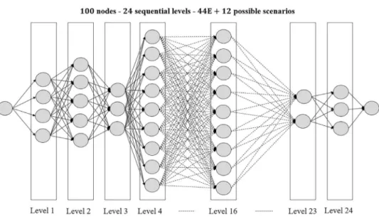
Fig. 6. The structure of the project model used for the experiments.
Table 1
A detailed description of the nominal values of the project graph nodes (part 1).
Level 1 2 3 4 5 6 7 8 9 10 11 12 Number of nodes 4 5 3 9 4 5 3 7 2 3 2 2 𝐶− min 𝑇𝑖 4870 20 760 1010 9580 24 580 2670 16 750 30 040 40 000 2670 3390 16 750 𝐶− max 𝑇𝑖 5500 23 120 1210 12 200 27 200 5930 18 930 32 430 43 000 5930 4215 18 930 𝐶−mean 𝑇𝑖 5185 21 940 1110 10 890 25 890 4300 17 840 31 235 41 500 4300 3802.5 17 840 𝐷− min 𝑇𝑖 11 45 3 30 30 2 21 59 80 2 2 21 𝐷max 𝑇𝑖 15 58 5 38 38 5 25 66 85 5 4 25 𝐷𝑇−mean 𝑖 11 45 3 30 30 2 21 59 80 2 2 21 𝑅min 𝑇𝑖 0.0344 0.1110 0.0196 0.0810 0.1272 0.0555 0.1165 0.1270 0.1044 0.0066 0.1614 0.0849 𝑅− max 𝑇𝑖 0.2504 0.1270 0.1348 0.2277 0.2160 0.2716 0.1824 0.1885 0.1695 0.0173 0.1948 0.2091 𝑅mean𝑇 𝑖 0.0344 0.111 0.0196 0.081 0.1272 0.0555 0.1165 0.127 0.1044 0.0066 0.1614 0.0849
as given in the following expressions:
𝐶𝑗𝑔−= ∑ 𝑖∈Path𝑓 𝑗 𝐶𝑖− (27) 𝐶𝑗𝑔+= ∑ 𝑖∈Path𝑓 𝑗 𝐶𝑖+ (28) 𝐷𝑗𝑔−= ∑ 𝑖∈Path𝑓 𝑗 𝐷−𝑖 (29) 𝐷𝑔+ 𝑗 = ∑ 𝑖∈Path𝑓 𝑗 𝐷+ 𝑖. (30)
All the task nodes visited by the ant 𝑓 before the node 𝑗 are belonging to the path Path𝑓
𝑗. The algorithm below gives a general structure of the MONACO algorithm. At the end of an iteration, when all the ants have reached the end node and deposited their pheromone trails, a Pareto-front is built and memorized. The new solutions obtained during the iteration are compared to the memorized Pareto-front. The dominated solutions are removed. In order to evaluate the performance of the
Table 2
A detailed description of the nominal values of the project graph nodes (part 2).
Level 13 14 15 16 17 18 19 20 21 22 23 24 Number of nodes 4 5 3 9 4 5 3 7 2 3 2 3 𝐶− min 𝑇𝑖 5250 4340 10 820 9580 2670 3945 17 640 30 040 2670 2670 215 210 𝐶− max 𝑇𝑖 15 030 23 120 20 760 26 700 27 200 18 930 32 430 53 000 4050 3390 324 258 𝐶𝑇−mean 𝑖 10 140 13 730 15 790 18 140 14 935 11 437.5 25 035 41 520 3360 3030 269.5 234 𝐷− min 𝑇𝑖 11 45 3 30 30 2 21 59 80 2 12 21 𝐷− max 𝑇𝑖 15 58 5 38 38 5 25 66 85 5 16 28 𝐷𝑇−mean 𝑖 11 45 3 30 30 2 21 59 80 2 12 21 𝑅min 𝑇𝑖 0.0023 0.0576 0.0543 0.0503 0.0725 0.1152 0.0719 0.0676 0.1348 0.1041 0.0691 0.0687 𝑅max 𝑇𝑖 0.1971 0.1585 0.2401 0.1713 0.1895 0.2619 0.1779 0.2404 0.1413 0.1812 0.1731 0.2162 𝑅mean 𝑇𝑖 0.0023 0.0576 0.0543 0.0503 0.0725 0.1152 0.0719 0.0676 0.1348 0.1041 0.0691 0.0687
Fig. 7. The hyper-volume, the mean performance and the standard deviation of mean performance for the MOACO and MONACO algorithms with 𝜌 = 0.03.
MONACO algorithm, the hyper-volume metric is computed within the objective space using the algorithm proposed inFonseca et al.(2006). More the volume is high, more the Pareto-front is good (i.e. near to the origin (0, 0, 0)). At the end of the iterations, the memorized Pareto-front constitutes the solution of our problem. The next step of the integrated process is the selection, by a decision maker of one scenario of the Pareto-front.
The framework of the optimization tool is represented inFig. 5. The tool, developed using the Ruby language, allowed to compare the performances of the standard MOACO (i.e. without learning) algorithm versus the MONACO one (i.e. with learning). The project graph model is defined in a first file named ‘‘Graph.rb’’. It contains the matrix of adjacent nodes and the set of triplets (𝐶, 𝐷, 𝑅) associated to the nodes. This file is the first input of the main program which is stored in the
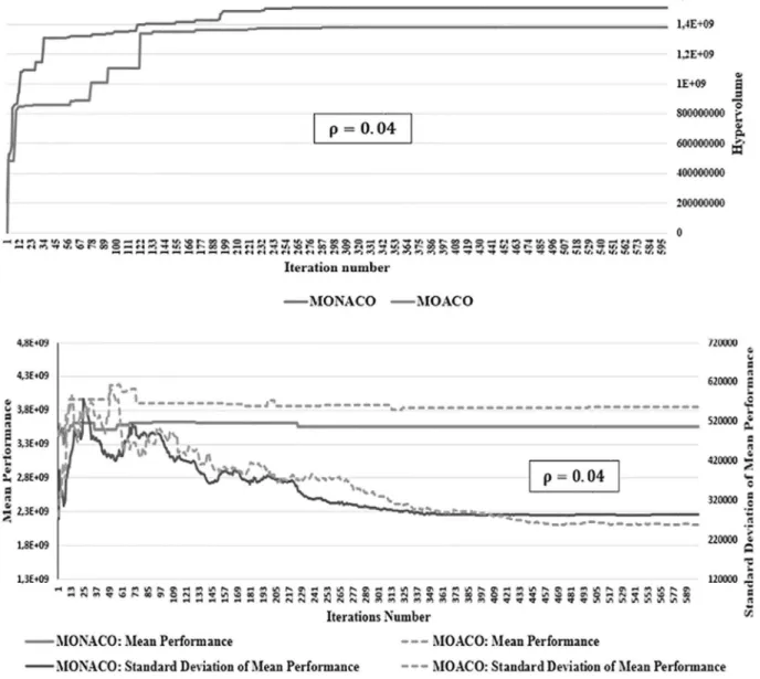
Fig. 8. The hyper-volume, the mean performance and the standard deviation of mean performance for the MOACO and MONACO algorithms with 𝜌 = 0.04.
file ‘‘MONACO.rb’’. The parameters of the algorithm are defined and stored into the file ‘‘Parameters.rb’’. The MONACO software calls the sub-program stored in the file Hypervolume.py (Python language — (Fonseca et al., 2006)) in order to compute the hyper-volume indicator. Finally, the output of the program is stored in the files ‘‘Results.csv’’ and ‘‘Pareto-front.csv’’. The former contains the hyper-volume, the mean performance, the standard deviation and the CPU time indicators for each iteration. They are stored for further analysis. The second file contains the solutions of the Pareto-front from where one solution can be selected in order to be scheduled.
5. Experiments
To validate our method, a set of experiments was done by consid-ering a project model composed by sequential levels. Each node of a level 𝑛 is connected with all the nodes of the level 𝑛 + 1. TheFig. 6
represents the structure of the considered project graph which has been used to attest the efficiency of the MONACO algorithm. This algorithm was developed by using the Ruby language and the experiments were
done on a desktop computer (Intel® Core™ i7 3,6 GHz processor). The
experiments aim to make a comparative analysis of the performances of the MOACO algorithm versus the MONACO algorithm.
The considered project graph includes 100 nodes with 24 sequential levels and each level has between 2 and 9 nodes. The combinations
for this instance give 44E+12 possible scenarios. TheTables 1 and
2 represent the minimal, the maximal and the mean values of the
nominal cost, duration and risk for the tasks. The maximal values of cost, duration and risk for each node are computed randomly between 10% and 50% above the nominal values. The values of risk are computed using the formulas 7 and 15 (GOWA operator with the parameter 𝑧 = 2). The initial parameter settings are given inTable 3and were evaluated empirically. The operator GOWA is used systematically with the value 𝑧 = 2(quadratic mean). Thus, this operator gives a greater weight to the largest values with regards to the lowest ones.
The colony has 200 ants and the number of iterations is 600. The value of the reference point to compute the hyper-volume above the Pareto-front for the triplet (cost, duration, risk) is [2E + 6, 1E + 3, 10]. It was evaluated from several experiments and corresponds to the upper bounds. To evaluate our method, three key performance indicators were considered to give a comparison between MOACO and MONACO algorithms. These indicators are the mean performance (Eq.(31)), the
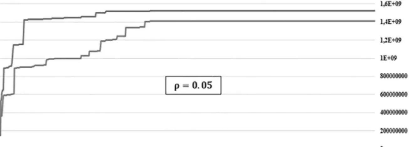
Fig. 9. The hyper-volume, the mean performance and the standard deviation of mean performance for the MOACO and MONACO algorithms with 𝜌 = 0.05.
standard deviation of mean performance (Eq. (32)) and the
hyper-volume corresponding to the Pareto-front. The mean performance and its standard deviation are computed from the mean values of costs, durations and risks of the Pareto-optimal solutions that are obtained at the end of each iteration. Thus, the Pareto-front is given at the end of each iteration when all the ants of the colony have reached the last node of the project graph and the hyper-volume is computed. The performance indicators are defined by:
MeanPerf = MeanC × MeanD × MeanR (31)
StdDevPerf = StdDevC × StdDevD × StdDevR. (32)
The set of experiments has demonstrated that the evaporation rate is the key parameter that impacts the most the results of MOACO and MONACO algorithms with regards to the other parameters. The performance of MOACO and MONACO algorithms does not change by varying the values of the parameters: 𝛼, 𝛽, 𝜏𝐶
0, 𝜏 𝐷 0, 𝜏 𝑅 0, 𝜑 𝐶, 𝜑𝐷, 𝜑𝑅, 𝑤𝐶, 𝑤𝐷, 𝐶𝑝𝐶0, 𝐶𝑝𝐷0, 𝜆𝐶0, 𝜆 𝐷 0, 𝜆 𝑅
0. Thus, a sensitivity analysis was
Table 3
Initial parameter settings.
Symbol Parameter Value
𝛼 Global attractiveness 1 𝛽 Local attractiveness 1 𝜌 Evaporation rate 0.05 𝜏𝐶 0, 𝜏 𝐷 0, 𝜏 𝑅
0 Initial quantities of pheromones 1
𝜑𝐶, 𝜑𝐷, 𝜑𝑅 Constants 1
𝑧 GOWA parameter 2 (quadratic mean)
𝑤𝐶, 𝑤𝐷 Weights
1 2
𝐶𝑝𝐶0 Initial capital of project cost [400 000, 425 000]
𝐶𝑝𝐷0 Initial capital of project duration [800, 825]
𝜆𝐶
0, 𝜆
𝐷
0, 𝜆
𝑅
0 Initial values of the dynamic weights 1 3
carried out specifically for 𝜌. Several experiments have been done using several values for 𝜌. TheFigs. 7–10represent the results obtained for 𝜌 = 0.03; 𝜌 = 0.04 ; 𝜌 = 0.05 and 𝜌 = 0.06. The experiments have shown that the value of 𝜌 that gives the best performance is 0.05. The curves are representing the performance with regard to the iteration number
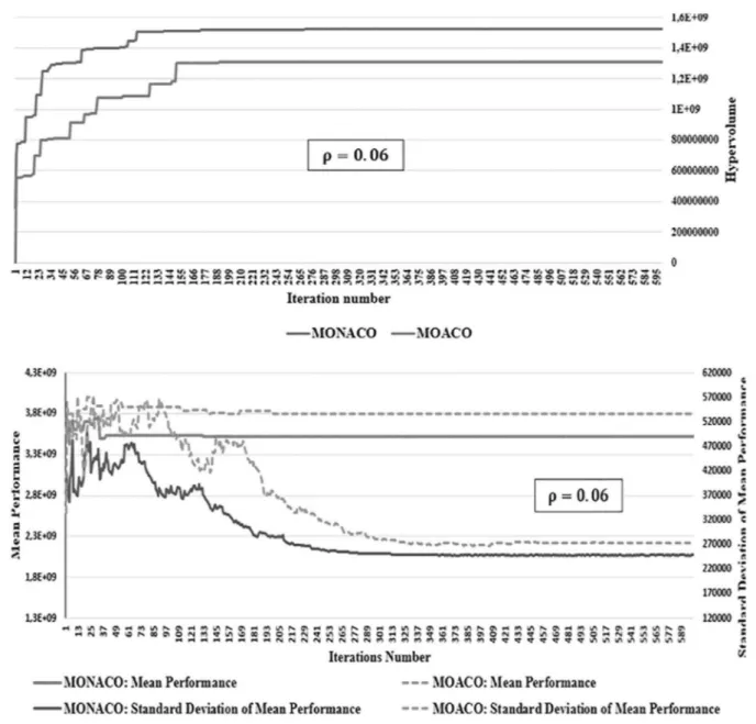
Fig. 10. The hyper-volume, the mean performance and the standard deviation of mean performance for the MOACO and MONACO algorithms with 𝜌 = 0.06.
following several values of 𝜌. It is noticed that for the value 𝜌 = 0.03 (cf.Fig. 7) the curve of the hyper-volume of the MOACO algorithm is above the MONACO one, which is the opposite of the intended goals. Moreover, the standard deviation of mean performance indicator does not point out the MONACO algorithm performance because its curve has many overlaps with the MOACO algorithm one. From the value of 𝜌 = 0.04, an improvement of the MONACO algorithm is clearly observed inFig. 8because the MONACO hyper-volume is greater than the MOACO
one. However,Fig. 9shows that the MONACO performance is better
for 𝜌 = 0.05 because the gap between the mean performance curves of both algorithms is greater. Furthermore, the standard deviation of mean performance curves keeps the same shape for 𝜌 = 0.04 until the iteration 403 where there is an overlap and a decrease performance of MONACO which is not the case for 𝜌 = 0.05. InFig. 10, for 𝜌 = 0.06 the results are close to those obtained with 𝜌 = 0.05. However, there is a decreasing performance for the MONACO algorithm whether for hyper-volume, mean performance or standard deviation of mean performance. That will lead to an overlap and then similar curves than those ofFig. 7
in the case of 𝜌 = 0.03. This sensitivity analysis of the parameter 𝜌 leads
us to conclude that the MONACO algorithm gives better results than the MOACO one when the values range of 𝜌 are between 0.05 and 0.06. Moreover, the best performance is less sensitive to the variation of 𝜌 for the MONACO algorithm. Thereby, it is easier to adjust the parameters in an industrial context. The performances of the algorithms with regards to CPU time for the value 𝜌 = 0.05 are detailed in the next paragraphs.
For 𝜌 = 0.05, a series of additional tests were carried out to make a comparison between both algorithms following the indicators of hyper-volume, mean performance and standard deviation of mean
performance. The results ofFig. 9show that the hyper-volume of the
MONACO algorithm is better than the hyper-volume of the MOACO one with almost a difference of 7.82% (iteration #600). Both algorithms performance stagnate after the iteration #240. From the iteration #240 to the iteration #600, the MOACO improves its hyper-volume of 0.3% versus 0.1% for the MONACO one. Moreover, the learning mechanism enables the MONACO algorithm to give better performances than the MOACO algorithm by increasing the mean performance with a difference of 12.51% and by decreasing the standard deviation of mean performance with a difference of 23.65%.
Table 4
Table of CPU times in seconds for the 10 tests for the MONACO Algorithm.
Iteration number 10 20 30 40 50 60 70 100 130 140 160 170 200 240 600
Hypervolume 890 642 686 947 871 755 1 149 311 836 1 422 666 426 1 426 123 046 1 428 867 640 1 432 494 547 1 442 342 824 1 447 460 092 1 458 533 506 1 498 707 710 1 515 063 602 1 519 452 484 1 520 277 323 1 521 363 454 Mean cost 308 800.0 309 773.0 310 606.0 311 951.0 313 088.0 312 375.0 310 364.0 313 185.0 319 519.0 319 219.0 319 809.0 320 133.0 322 411.0 323 241.0 325015.0 Mean duration 664.0 660.0 661.0 660.0 659.0 659.0 660.0 660.0 659.0 659.0 660.0 660.0 661.0 662.0 662.0 Mean risk 10.73 10.55 10.34 10.11 10.03 9.98 9.99 9.75 9.36 9.34 9.16 9.09 8.92 8.78 8.67 Standard deviation of cost 22 557.09 22 569.69 24 539.72 24 392.26 25 160.27 24 916.18 23 755.32 23 679.95 23 068.47 22 411.16 21 306.61 20 617.6 20 756.85 20 386.96 20 241.14 Standard deviation of duration 18.13 15.16 14.72 15.4 14.48 14.26 13.86 13.56 13.16 13.19 12.78 12.16 11.98 11.79 11.37 Standard deviation of risk 1.3 1.22 1.27 1.16 1.13 1.15 1.14 1.23 1.18 1.18 1.17 1.14 1.17 1.12 1.09 Mean performance 3 457 830 758 3 603 474 854 3 497 820 732 3 407 189 811 3 447 149 035 3 447 149 035 3 403 142 877 3 408 402 758 3 408 402 758 3 408 402 758 3 408 402 758 3 408 402 758 3 408 402 758 3 408 402 758 3 408 402 758 Standard deviation of mean performance 530 911 418 531 458 007 435 072 412 553 408 596 376 254 395 058 358 504 349 429 318 143 286 669 290 565 270 435 250 354 Mean CPU time 2.46 4.92 7.35 9.74 12.14 14.57 17.01 24.30 31.71 34.25 39.16 41.71 49.44 59.43 149.54
Table 5
Table of CPU times in seconds for the 10 tests for the MOACO Algorithm.
Iteration number 10 20 30 40 50 60 70 100 130 140 160 170 200 240 600
Hypervolume 588 744 127 602 958 977 895 577 682 899 693 513 902 803 403 919 900 115 920 998 567 996 047 256 997 210 532 1.027E+09 1.079E+09 1.199E+09 1.243E+09 1.406E+09 1.411E+09 Mean cost 308 668.0 304 109.0 305 749.0 307 143.0 305 962.0 302 867.0 301 970.0 303 178.0 301 862.0 303 230.0 302 742.0 303 112.0 302 467.0 301 993.0 303 989.0 Mean duration 659.0 660.0 659.0 658.0 658.0 658.0 659.0 657.0 658.0 657.0 658.0 658.0 659.0 661.0 663.0 Mean risk 11.45 11.43 11.21 11.18 11.19 11.23 11.18 10.91 10.78 10.69 10.53 10.47 10.29 10.05 9.52 Standard deviation of cost 23 308.88 22 625.0 22 567.51 24 691.34 24 520.1 24 760.66 25 011.63 23 733.6 22 997.16 24 084.35 23 152.22 22 794.45 21 956.12 20 675.43 18 818.51 Standard deviation of duration 12.12 14.11 14.89 16.34 15.02 16.73 17.71 15.49 16.09 14.91 14.6 14.4 14.44 13.85 12.05 Standard deviation of risk 1.36 1.42 1.38 1.49 1.55 1.5 1.48 1.5 1.42 1.49 1.49 1.46 1.52 1.5 1.37 Mean performance 3.904E+09 3.929E+09 4.031E+09 3.936E+09 3.995E+09 4.155E+09 4.125E+09 3.977E+09 3.977E+09 3.977E+09 3.977E+09 4.022E+09 3.965E+09 3.835E+09 3.835E+09 Standard deviation of mean performance 383 760 454 393 463 124 600 001 570 876 622 639 655 539 552 939 526 146 536 103 502 115 479 802 481 110 429 682 309 568 Mean CPU time 1.73 3.44 5.12 6.81 8.50 10.19 11.88 16.97 22.04 23.74 27.14 28.84 33.95 40.76 102.96
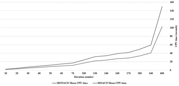
A deeper comparative analysis between MOACO and MONACO algorithms was considered to attest the advantage of using a learning mechanism. Thus, among the ten tests done above for 𝜌 = 0.05, the CPU time (in seconds) was measured for a representative sample of fifteen iterations and for the ten considered tests. The chosen iterations are determined according to the variations of the hyper-volume values in Fig. 9. For example, both algorithms stabilize after the iteration #240 which means that they stopped converging. Thus, the CPU time for the next iterations are not represented except for the last
one. TheFig. 11 represents the mean CPU time with regards to the
iterations for the MOACO and MONACO algorithms. It shows that the MONACO algorithm runs in a reasonable amount of time compared to
the MOACO algorithm. Indeed, regarding the hyper-volume indicator, a better convergence speed is observed for the MONACO algorithm than for the MOACO one. At the iteration #40, the MONACO algorithm gives almost the same performance level (hyper-volume = 1.422E+9) than the MOACO one at the iteration #240 (hyper-volume = 1.406E+9).
Regarding the CPU times (cf.Tables 4and5), the MONACO algorithm
reaches this performance (iteration #40) in less than 10 s versus 40 s for the MOACO one to reach the iteration #240. The best performance level is obtained at the iteration #240 for both. The MOACO reaches the iteration #240 in 40 s versus 60 s for the MONACO one. The learning mechanism needs 50% of extra time to reach the best performance but this performance is 8.12% better for the hyper-volume and 12.5% better
Fig. 11. Comparison of mean CPU time between MONACO and MOACO algorithm.
for the mean performance. However, this performance is obtained in less than one minute which is acceptable in a decision making context if we consider that the problem size used for the tests is huge (44𝐸 + 12 solutions).
6. Conclusion
In this paper, the integration of the standard industrial processes existing in the literature (system engineering and project management processes) in a global process was described. At first, a detailed version of this proposed integrated process was described by defining the functioning of the various sub-processes and actors involved in the project. This process is fed by knowledge and/or experience bases as well as by experts. It is supported mainly by the multi-criteria decision support tool based on the MONACO algorithm that optimize three objectives of the triplet (cost, duration, risk). The experiments done with a model of a large project graph have shown that the MONACO algorithm gives better results in a reasonable computational time with the learning mechanism than the MOACO one.
Compared to the standard ACO approaches, the proposed MONACO algorithm uses dynamic weights to take into account the paths taken by each ant using the initial consumed capitals of cost, duration and risk. Another specificity of this algorithm is the consideration of risk as a third objective to optimize besides cost and duration which is an overall view of risk in the MONACO algorithm. Moreover, the proposed approach developed in this article is very useful to engineers, project managers, risk managers, etc. It allows to select, at the earliest phases of a system engineering project, one Pareto-optimal project scenario that will be scheduled and realized. The integrated process provided with its optimization tool allows:
– The collaboration of every actor, stakeholders and the decision maker in the definition of the decision space (construction of the project graph),
– To favorize the collaboration work and the synchronization that is required between project managers and system engineers, – To take into account very early (and before the selected project
scenario scheduling and realization) the potential risks with their impacts on costs and durations,
– A good level of acceptance in companies because of the full compliance with the standard industrial processes.
Uncertainty on tasks costs and durations is modeled as simple intervals. Nevertheless, the current risk modeling as simple intervals on cost and duration could be improved. A more developed representation of risk will be considered by exploring other risk modeling methods. In the proposed approach, the actors of the different processes have to build the graph of project in a cooperative way. The representation of risks is done by modeling directly their impacts on nominal durations and costs. Therefore, the intervals are built from this kind of analysis which can be time consuming and need experts to be done. In order to improve this work, a probabilistic causal model representing the risks and their impacts on costs and durations could be more easy than the interval definitions. The results could be, for every task of the graph, a distribution of probabilities of the different values (costs and durations). This kind of model could be more representative of the real industrial context and more easy to build by the actors of processes. Therefore, one of the near perspectives of this work is to propose such a model and to integrate it into our integrated process as well as in the MONACO algorithm.
References
Abdallah, H., Emara, H.-M., Dorrah, H.-T., Bahgat, A., 2009. Using ant colony optimization algorithm for solving project management problems. Expert Syst. Appl. 36 (6), 10004– 10015.
Abeille, J., Coudert, T., Vareilles, E., Geneste, L., Aldanondo, M., Roux, T., 2010. Formal-ization of an integrated system/project design framework: first models and processes. In: 1st International Conference on Complex Systems Design & Management, Paris (France).
Acebes, F., Pajares, J., Galán, J.M., López-Paredes, A., 2013. Beyond earned value man-agement: A graphical framework for integrated cost, schedule and risk monitoring. Proc.-Soc. Behav. Sci. 74, 181–189.
Aghaie, A., Mokhtari, H., 2009. Ant colony optimization algorithm for stochastic project crashing problem in PERT networks using MC simulation. Int. J. Adv. Manuf. Technol. 45, 1051–1067.
Aqlan, F., Ali, E.-M., 2014. Integrating lean principals and fuzzy bow-tie analysis for risk assessment in chemical industry. J. Loss Prev. Process Ind. 29, 39–48.
Aven, T., 2016. Risk assessment and risk management: Review of recent advances on their foundation. European J. Oper. Res. 253 (1), 1–13.
Baroso, P., Coudert, T., Villeneuve, E., Geneste, L., 2014. Multi-objective optimization and risk assessment in system engineering project planning by Ant Colony Algorithm. In: 2014 IEEE International Conference on Industrial Engineering Management, pp. 438–442 Kuala-Lumpur, Malaysia.
Béler, C., Desforges, X., 2007. Experience feedback, from cases to knowledge. In: The 4th International Federation of Automatic Control Conference on Management and Control of Production and Logistics (MCPL 2007), Sibiu (Romania).
Better, M., Glover, F., 2008. Simulation Optimization: applications in risk management. Int. J. Inf. Technol. Decis. Mak. 7 (4), 571–587.
Chen, W.-N., Zhang, J., 2012. Scheduling multi-mode projects under uncertainty to optimize cash flows: A Monte Carlo ant colony system approach. J. Comput. Sci. Tech. 27 (5), 950–965.
Chen, W.-N., Zhang, J., 2013. Ant colony optimization for software project scheduling and staffing with an event-based scheduler. IEEE Trans. Softw. Eng. 39 (1), 1–17. Coudert, T., Vareilles, E., Aldanondo, M., Geneste, L., Abeille, J., 2011. Synchronization
of system design and project planning: Integrated model and rules. In: 5th Interna-tional Conference on Software, Knowledge Information, Industrial Management and Applications (SKIMA). University of Sannio Benevento (Italy).
Dorigo, M., Birattari, M., Stützle, T., 2006. Ant colony optimization, artificial ants as a computational intelligence technique. IEEE Comput. Intell. Mag.
Dorigo, M., Stützle, T., 2010. Ant colony optimization: Overview and recent ad-vances. In: Gendreau, M., Potvin, Y. (Eds.), Handbook of Metaheuristics, second ed. In: International Series in Operations Research & Management Science, vol. 146, Springer Verlag, New York, pp. 227–263.
Fan, M., Lin, N.-P., Sheu, C., 2008. Choosing a project risk-handling strategy: An analytical model. Int. J. Prod. Econ. 112 (2), 700–713.
Fang, C., Marle, F., 2012. A simulation-based risk network model for decision support in project risk management. Decis. Support Syst. 52 (3), 635–644.
Fang, C., Marle, F., Zio, A., Bocquet, J.-C., 2012. Network theory-based analysis of risk interactions in large engineering projects. Reliab. Eng. Syst. Saf. 106, 1–10. Fernandez, E., Gomez, C., Rivera, G., Cruz-Reyes, L., 2015. Hybrid metaheuristic approach
for handling many objectives and decisions on partial support in project portfolio optimization. Inform. Sci. 315, 102–122.
Flage, R., Aven, T., Zio, E., Baraldi, P., 2014. Concerns, challenges, and directions of development for the issue of representing uncertainty in risk assessment. Risk Anal. 34 (7), 1196–1207.
Fonseca, C.M., Paquete, L., Lopez-Ibanez, M., 2006. An improved dimension-sweep algo-rithm for the hypervolume indicator. In: IEEE Congress on Evolutionary Computation, pp. 1157–1163, Vancouver (Canada).
Galloway, P.D., 2006. Survey of the construction industry relative to the use of CPM scheduling for construction projects. J. Constr. Eng. Manage. 132 (7), 697–711. Jun-Yan, L., 2012. Schedule Uncertainty control: A literature review. Physics Procedia 33,
1842–1848.
Kamsu Foguem, B., Coudert, T., Béler, C., Geneste, L., 2008. Knowledge formalization in experience feedback processes: An ontology-based approach. Comput. Ind. 59 (7), 694–710.
Kaya, I., Karhaman, C., 2010. Development of fuzzy process accuracy index for decision making problems. Spec. Issue Model. Uncertainty 180 (6), 861–872.
Khodakarami, V., Fenton, N., Neil, M., 2007. Project scheduling: Improved approach to incorporate uncertainty using Bayesian Networks. Proj. Manage. J. 38, 39–49.
Lachhab, M., Béler, C., Solano-Charris, E.L., Coudert, T., 2017. Towards an Integration of System Engineering and Project Risk Management Processes for a Decision Aiding Purpose. In: The 20th World Congress of the International Federation of Automatic Control (IFAC 2017 World Congress), Toulouse (France).
Lachhab, M., Coudert, T., Béler, C., 2016. Scenario selection optimization in System Engineering Projects under uncertainty: A multi-objective Ant Colony method based on a learning mechanism. In: Proceedings of the IEEE International Conference on Industrial Engineering and Engineering Management (IEEM), Bali (Indonesia).
Nguyen, T.-H., Marmier, F., Gourc, D., 2013. A decision-making tool to maximize chances of meeting project commitments. Int. J. Prod. Econ. 142 (2), 214–224.
Pearl, J., 1995. Probabilistic reasoning in intelligent systems: Networks of plausible inference. Synth.-Dordr. J. 104 (1), 162.
Pitiot, P., Coudert, T., Geneste, L., Baron, C., 2010. Hybridization of bayesian networks and evolutionary algorithms for multi-objective optimization in an integrated product design and project management context. Eng. Appl. Artif. Intell. 33 (5), 830–843. PMBOK Guide, 2013. A Guide To the Project Management Body of Knowledge, fifth ed.
Project Management Institute.
Ramageri, M., Bharati, M., 2010. Data mining techniques and applications. Indian J. Comp. Sci. Eng. 1 (4), 301–305.
SEBOK Guide, 2014. A Guide To the System Engineering Body of Knowledge, Version1.3. The Trustees of the Stevens Institute of Technology.
Stützle, T., López-Ibáñez, M., Dorigo, M., 2011. A concise overview of applications of ant colony optimization. In: Wiley Encyclopedia of Operations Research and Management Science.
Vareilles, E., Coudert, T., Aldanondo, M., Geneste, L., Abeille, J., 2015. System design and project planning: Model and rules to manage their interactions. Integr. Comput.-Aided Eng. 22 (4), 327–342.
Villeneuve, E., Béler, C., Peres, F., Geneste, L., Reubrez, E., 2016. Decision-support methodology to assess risk in end-of-life management of complex systems. IEEE Syst. J. (ISSN: 1932-8184) 99, 1–10.
Ward, S., Chapman, C., 2003. Transforming project risk management into project uncer-tainty management. Int. J. Proj. Manage. 21 (2), 97–105.
Yager, R., 2004. Generalized OWA aggregation operators. Fuzzy Optim. Decis. Mak. 3 (1), 93–107.