DISTRIBUTION SPATIALE DES COMMUNAUTÉS DE VERS DE TERRE ET LEUR EFFET SUR LES GAZ À EFFET DE SERRE EN CHAMPS AGRICOLES ET EN BANDES
RIVERAINE FORESTIÈRES
par
Ashley Cameron
Mémoire présenté au Département de biologie en vue de l’obtention du grade de maître ès sciences (M.Sc.)
FACULTÉ DES SCIENCES UNIVERSITÉ DE SHERBROOKE
Le 17 mars 2020
le jury a accepté la thèse de Madame Ashley Cameron dans sa version finale.
Composition du jury
Professeur Robert Bradley Directeur de recherche
Département de biologie, Université de Sherbrooke
Professeure Joann Whalen Codirectrice de recherche
Département des sciences des ressources naturelles, Collège Macdonald de l’Université de McGill
Professeur Naresh Thevathasan Évaluateur externe
Université de Guelph
Professeur John William Shipley Évaluateur interne
SUMMARY
This thesis reports the findings from a research project that aimed to determine the effect of earthworms on greenhouse gas (GHG) emissions in forested riparian buffer strips (FRBS). This project had two research questions. Firstly, we wanted to determine how earthworms are distributed in agricultural ecosystems and whether they had a preference for FRBS over adjacent agricultural fields. Secondly, we wanted to determine the effect of earthworms on the emission of the three most prominent GHG (CO2, N2O and CH4) and how the effect of earthworms is affected
by soil characteristics, namely, soil origin and soil texture. We expected earthworms to have a preference for FRBS and for them to have a positive effect on GHG emissions.
For the first research question, we conducted a field survey on agricultural fields with adjacent FRBS in Southern Quebec and Ontario as well as in the Czech Republic. At each site, we quantified earthworm numbers from each functional group (anecic, endogeic and epigeic) and characterized the site by noting the percentage coverage of the different types of vegetation and analysing soil’s physicochemical properties. We found that for Eastern Canada, earthworm numbers, organic matter and soil moisture were all higher in FRBS than in adjacent agricultural fields. However, in Czech Republic, earthworm numbers were higher in agricultural fields than FRBS and there was no significant difference in moisture between agricultural fields and FRBS. This indicated that moisture is an important variable in predicting the distribution of earthworms. Furthermore, we found that earthworm numbers are positively associated with organic matter, pH, clay content and the percent coverage of deciduous trees and negatively associated with sand content and the percent coverage of coniferous trees. Following these results, the next step was to determine what effect earthworms have on GHG emissions.
In order to determine the effect of earthworms on GHG emissions we conducted controlled microcosm experiments. These experiments were conducted using a replicated factorial design
comprising of 3 soil origins (deciduous FRBS, coniferous FRBS, agricultural field) x 2 soil textures (field conditions, high clay) x 3 earthworm life habits (anecic, endogeic, no earthworm). Soils originating from FRBS emitted more CO2 than soils from agricultural fields with soils from
deciduous stands having higher emissions than soils from coniferous stands. Soils with a higher clay content emitted less CO2 than soils with a lower clay content. Soils with earthworms emitted
more CO2 than soils without earthworms, however, this effect diminished with time and was no
longer significant after ten weeks. Additionally, soils with earthworms emitted more N2O than
soils without earthworms. For CH4, the transformation rates were higher for soils from FRBS than
soils from agricultural fields under both anaerobic and aerobic conditions.
With earthworms having an overall positive effect on GHG emissions, FRBS should be designed such that they prevent the establishment of earthworms. Therefore, coniferous trees would be preferable over deciduous trees. Firstly, earthworm numbers were shown to be negatively associated with coniferous tree coverage, and, in the event that earthworms do become established, GHG emissions were shown to be lower from coniferous soils than deciduous stands.
SOMMAIRE
Cette mémoire rapporte sur un projet de recherche qui visait à déterminer l’effet des vers de terre sur les gaz à effet de serre en bandes riveraines forestières. Cela consistait de deux questions de recherche. Premièrement, nous voulions déterminer comment les vers de terre sont distribués en milieux agricoles et s’ils ont une préférence pour les bandes riveraines forestières comparé aux champs agricoles adjacents. Deuxièmement, nous voulions savoir l’effet des vers de terre sur les principaux gaz à effet de serre (CO2, N2O et CH4) et comment cela interagit avec les
caractéristiques de sols, notamment, la texture du sol et la provenance, soit sous une plantation de feuillus, conifères ou un champ agricole. Nous prévoyons que les vers de terre auront une préférence pour les bandes riveraines forestières et qu’ils auront un effet positif sur les émissions des gaz à effet de serre.
Pour la première question de recherche, nous avons échantillonné des champs agricoles ayant des bandes riveraines forestières adjacentes situées à travers du sud de l’Ontario et du Québec ainsi qu’en République Tchèque. À chaque site nous avons quantifié le nombre de vers de terre de chaque groupe fonctionnel (endogé, epigé et anécique) et avons caractérisé le site en notant le pourcentage de recouvrement des strates végétales et en analysant un échantillon de sols pour des caractéristiques physico-chimiques. Nous avons trouvé que l’abondance des vers de terres et l’humidité et le pourcentage de matière organique du sol étaient plus élevés en bande riveraines forestières qu’en champs agricoles au Canada. Par contre, en République Tchèque l’abondance des vers de terre était plus élevée dans les champs agricoles et il n’y avait pas de différence d’humidité entre les sols des bandes riveraines et ceux des champs agricoles. Cela indique que l’humidité est très importante dans la détermination de la distribution des vers de terres. De plus, nous avons déterminé que le nombre de vers de terre est positivement associé au pourcentage de matière organique, le pH et le pourcentage d’argile du sol, le pourcentage de recouvrement des arbres feuillus et est négativement associé au pourcentage de sable du sol et le pourcentage de
recouvrement des conifères. Suivant ces conclusions, nous devions déterminer leur effet sur les gaz à effet de serre.
Pour la deuxième question de recherche, nous avons complété deux expériences en microcosmes pour déterminer l’effet des vers de terre sur les émissions de gaz à effet de serre. Ces expériences avaient 18 traitements comprenant une série factorielle de trois provenances de sols (bande riveraine feuillu, bande riveraine conifère et champ agricole), deux textures de sols (argile élevé et argile bas) et trois niveaux de vers de terre (anécique, endogé et aucun). Les sols de bandes riveraines ont émis plus de CO2 que les sols de champs agricoles avec les sols feuillus ayant des
émissions plus élevées que les sols conifères. Les sols avec l’argile élevé ont émis moins de CO2
que les sols avec moins d’argile. Les sols avec des vers de terres ont émis plus du CO2 que les sols
sans vers de terres, mais cet effet a diminué avec le temps et n’était plus significatif après dix semaines. Les sols avec des vers de terres ont aussi émis plus de N2O que les sols avec aucun vers
de terre. Pour le CH4, l’origine du sol était le facteur le plus important avec les sols de bandes
riveraines ayant des taux de transformation de CH4 plus élevés que les sols agricoles sous
conditions aérobiques et anaérobiques.
Étant donné que les vers de terre augmentent les émissions de gaz à effet de serre, des bandes riveraines comprenant des conifères au lieu des feuillus serait préférable pour éviter l’établissement des vers de terres. De plus, les émissions de gaz à effet de serre sont moins élevées dans les sols de conifères alors l’effet des vers de terre serait plus basse s’ils réussissent à coloniser les bandes riveraines.
ACKNOWLEDGEMENTS
I would first like to thank my supervisor Professor Robert Bradley of the Biology Department at Université de Sherbrooke. Throughout this project he allowed this paper to be my own work while guiding me in the right direction as I needed it. I would also like to thank my co-supervisor, Professor Joann Whalen, as well as the members of my supervisory committee, Professor Bill Shipley and Professor Naresh Thevathasan, whose support throughout this project kept me on the right track.
I would like to thank Dr. Bill Parsons for his guidance on laboratory analyses, Dr. Agnieszka Józefowska for her instruction on identifying foreign earthworms, as well as Miloslav Šimek for the donation of this laboratory and time which made our work in the Czech Republic possible. I would also like to acknowledge the number of students who assisted with the field work component of this project: Petra Benetková, Gabriel Boilard, Anne Bolduc, Raphaëlle Dubois, Marika Caoutte, Brent Coleman and Laurence Guay.
This project would not have been possible without the financial support of Agriculture and Agri-Food Canada’s Agricultural Greenhouse Gas Program (AGGP) and Centre Sève’s AgroPhytoSciences scholarship program.
TABLE OF CONTENTS
SUMMARY ……….. iv
SOMMAIRE ………. vi
List of abbreviations ………....…..… xi
List of tables ………...………...… xii
List of figures ………...………..….…… xiii
CHAPTER 1: GENERAL INTRODUCTION ……….….. 1
CHAPTER 2: THE DISTRIBUTION OF EARTHWORMS IN AGROECOSYSTEMS WITH FORESTED RIPARIAN BUFFER STRIPS AS EXPLAINED BY SOIL AND SITE CHARACTERISTCS ……….….. 14
2.0 Abstract ………...………. 15
2.1 Introduction ………..……… 16
2.2 Materials and methods ………..… 18
2.2.1 Study sites ……….… 18
2.2.2 Experimental design and field sampling ………... 19
2.2.3 Soil analyses and earthworm identification ………..…. 20
2.2.4 Statistical analyses ……… 21
2.3 Results ………..……… 23
2.4 Discussion ………..……….. 30
2.5 Acknowledges ……….……. 34
2.6 References ……… 35
CHAPTER 3: THE EFFECT OF EARTHWORMS AND SOIL CHARACTERISTICS ON GREENHOUSE GAS EMISSIONS IN FORESTED RIPARIAN BUFFER STRIPS ………. 40
3.0 Abstract ……… 41
3.1 Introduction ……….……. 42
3.2 Materials and methods ………..…… 45
3.2.2 Gas sampling and analyses ………...………. 48
3.2.2.1 CO2 production and denitrification …..………..………. 48
3.2.2.2 Gross transformation rates and CH4 ………..……….…. 48
3.2.3 Soil analyses ………. 50
3.2.4 Statistical analyses ……...……….………..….. 51
3.3 Results ……….…. 51
3.3.1 CO2 production ……….……..……...………..……. 51
3.3.2 Nitrogen mineralization and denitrification …………..…...….………... 52
3.3.3 Gross CH4 transformation rates under aerobic and anaerobic headspaces ……….………...………...……….………... 53
3.4 Discussion ……… 55
3.5 Acknowledgments ……… 57
3.6 References ……… 58
CHAPTER 4: GENERAL DISCUSSION AND CONCLUSION ………..……….. 63
LIST OF ABBREVIATIONS
FRBS: forested riparian buffer strips GHG: greenhouse gas
CO2: carbon dioxide
N2O: nitrous oxide
LIST OF TABLES
Table 1 Ash-free dry mass estimates for earthworm species 21 Table 2
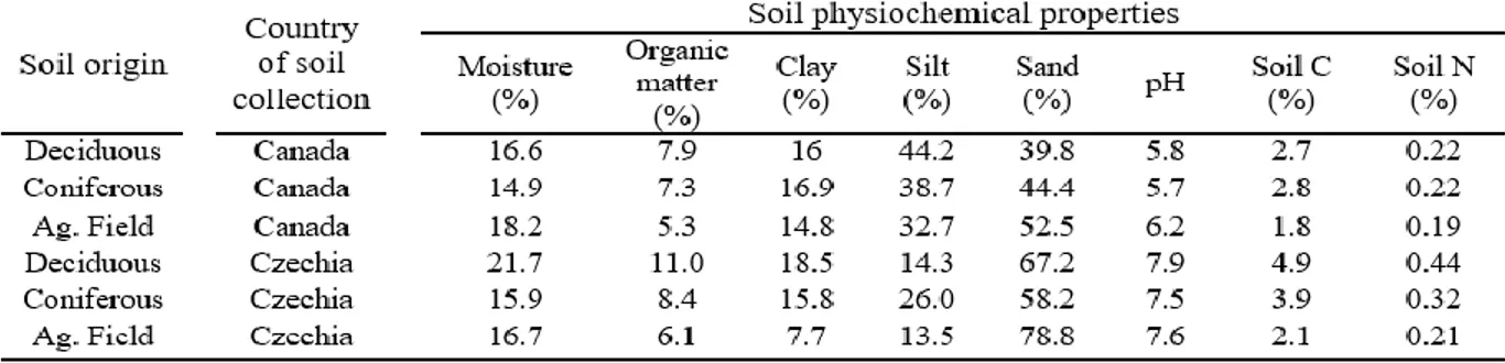
Physiochemical properties averaged over the five replicates for each of the three soil origins collected prior to microcosm assembly
LIST OF FIGURES
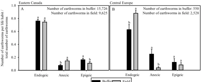
Figure 1 Proportion of earthworms by life habit in fields and buffers in (A) Eastern Canada and (B) Central Europe
24 Figure 2 Comparison of earthworm numbers, soil moisture and soil
organic matter in fields and buffers
25 Figure 3 Earthworms abundance and biomass in different stand
types in Eastern Canada and Central Europe
26 Figure 4 Results of distance-based redundancy using earthworm
species as the response variables and the percent coverage of vegetation types as explanatory variables
28
Figure 5 Results of regression tree analysis in Eastern Canada using earthworm abundance as response variable and soil and site characteristics as explanatory variables
29
Figure 6 Results of regression tree analysis in Central Europe using earthworm abundance as response variable and soil and site characteristics as explanatory variables
30
Figure 7 Mean CO2 flux (nmoles g-1 h-1) as affected by (A) soil
origin, (B) soil texture and (C) Earthworms
52 Figure 8 Mean N2O flux (nmoles g-1 h-1) as affected by earthworms 53
Figure 9 Mean gross production rate of CH4 (nmoles g-1 h-1) under
anaerobic headspace as affected by (A) soil origin, mean consumption rate of CH4 under anaerobic headspace as
affected by soil origin (B), mean gross production rate of CH4 under aerobic headspace as affected by soil origin (C)
and mean gross consumption rate of CH4 under aerobic
headspace as affected by soil origin (D)
CHAPTER 1
GENERAL INTRODUCTION
Agricultural contaminants constitute the most important factor contributing to the degradation in water quality in the United States. These contaminants originate from a number of sources such as pesticides, nutrients and sediments (Maas et al., 1984; U.S. Department of Agriculture, 1985). Several approaches have been implemented to mitigate the negative impacts of agricultural practices. One such practice is the planting or preservation of forested riparian buffer strips (FRBS). These FRBS can be defined as streamside ecosystems that are managed with the aim of enhancing water quality by controlling nonpoint source pollution and protecting the stream environment (Lowrance et al., 1997). In practice, planting trees in riparian environments has been widely recognized as a means to improve stream habitats and water quality (Parkyn et al., 2005) due to their ability to moderate stream temperatures, reduce the input of sediments, provide sources of organic matter and stabilize the stream bank (Osborne and Kovacic, 1993). Furthermore, FRBS can be effective at intercepting and absorbing large amounts of nitrogen that would otherwise enter the adjacent water body and cause significant stress to the aquatic ecosystem (Mayer et al., 2007; Fortier et al., 2010).
While the focus tends to be on improvements to water quality, FRBS also provide a number of additional environmental benefits. Streams and the associated riparian habitats play a vital role in structuring vertebrate communities, making the design of FRBS a key wildlife management issue for human-impacted environments (Anderson et al., 2004). Riparian zones provide habitats for fish, plants and wildlife with FRBS serving as landscape corridors by connecting habitats (Palone and Todd, 1997; National Research Council, 2002). Furthermore, while the planting of FRBS may decrease crop land, there is the potential for economic returns as FRBS provide woody materials to farmers resulting in income from timber (Schultz et al., 1995). With
this wide array of environmental benefits, FRBS strips have become widespread in agroecosystems. However, in order to objectively asses the net environmental benefits of FRBS, we also need to identify the potential downsides of FRBS. One criterion of particular interest is the effect of FRBS on greenhouse gas (GHG) emissions. Namely, are they serving as a source or sink for GHG emissions?
The rising atmospheric concentrations of GHGs made the identification of potential GHG sources and sinks an area of great importance. In 2013, the concentration of atmospheric CO2
surpassed 400 ppm for the first time in recorded history and current trends project that it will continue rising up to 1500 ppm (NASA, 2019). The concentration of CH4 is increasing at a rate
of approximately 2 % per year (Ramussen and Khalil, 1981), and, with CH4 having 21 times the
global warming potential of CO2 (Nicks et al., 2003), this can lead to an additional 0.4 ºK
increase in the earth’s surface temperature over the next 40 – 50 years (Ramussen and Khalil, 1981; Wang et al., 1976). Since the 1800s, the relative concentration of N2O to air has increased
by almost 20 %. Over recent decades, the atmospheric concentration of N2O has been increasing
at a rate of approximately 0.25 % per year, and these trends are expected to continue (Wuebbles, 2009). This rise is of significant concern since N2O has a warming potential 310 times greater
than that of CO2 (Nicks et al., 2003). With their rising concentrations and global warming
potential, these three gases – CO2, N2O and CH4 – can be thought of as the three most prominent
GHGs, making them the focus of this study.
Soils can serve as a major source or sink for the three most prominent GHGs. Approximately 20 % of global CO2 emissions originate from the soil (Rastogi and Pathak, 2002), as well as
about one third of CH4 and two thirds of N2O emissions (Smith et al., 2003). Consequently, is
assessing the rise in atmospheric GHG it will be necessary to study factors that will affect soil GHG emissions. These GHGs are released from the soil as a result of a number of biotic processes, namely respiration for CO2, methanogenesis for CH4 and a combination of
the factors that control these GHG producing processes will be of significant importance when assessing the ability of FRBS to limit soil GHG emissions. These factors include substrate availability (e.g. labile carbon or mineral nitrogen in the case of N2O), and soil physico-chemical
properties (e.g. pH and moisture), which will ultimately dictate microbial activity. Both substrate availability and soil physio-chemical properties may be significantly affected by earthworms (Lubbers et al., 2013). Consequently, the presence of earthworms is yet another factor that will need to be studied to determine the GHG balance of FRBS.
Earthworms have been deemed ecosystem engineers due to their ability to greatly modify the environments that they inhabit. For example, their feeding, burrowing and casting activities can change the soil structure, redistribute organic matter and alter the habitat of the microorganisms inhabiting the soil (Brown and Lavelle, 2000; Lavelle et al., 1997; Neilson and Hole, 1964). The resulting physical changes to the soil will influence processes at the ecosystem level, including: carbon storage, nitrogen transformation rates and the loss of nutrients via pore spaces (Bohlen et al., 2004). Additionally, these changes will affect the aforementioned regulatory process that control soil GHG emissions. As such, the presence of earthworms will be an essential component in studying the GHG balance in FRBS. Furthermore, the changes made by earthworms to the soil structure may negatively affect the ability of FRBS to perform environmental services. Although earthworms have been praised for improving soil structure and fertility (Fonte et al. 2019), both of these benefits are irrelevant in FRBS. Conversely, the burrowing activities of earthworms produce soil macropores, which create preferential flow pathways and increase the leaching of nutrients into adjacent streams (Schneider et al. 2017) thereby decreasing the ability of FRBS to sequester agricultural runoff. In order to propose an optimal FRBS design that minimizes the negative effects of earthworms, this study has been divided into two research questions.
Firstly, we need to determine how earthworms are distributed in agroecosystems. More specifically, are earthworms more abundant in FRBS than in adjacent agricultural fields? This
will involve determining which environmental characteristics drive the distribution of earthworms in order to predict earthworm abundance, and community composition, in both agricultural fields and FRBS. If earthworms are deemed to have a net negative effect on FRBS, then this data can be used to propose a design that will repel earthworms. Secondly, once we know how earthworms are distributed, we need to determine what effect they have on GHG emissions. Within the context of studying their effects in FRBS, we will need to determine how the earthworms’ ability to affect GHG emissions interacts with the soils that they are inhabiting. More specifically, how does the earthworm effect interact with soil origin and soil texture?
Before separating these two questions, one element that will play an important role in both research questions is earthworm life habit. Earthworms are divided into three groups (anecic, endogeic and epigeic) based on their lifestyle. The differences among these three groups may lead to different selection criteria for optimal habitats, and will affect the degree and manner in which earthworms alter the soil. Anecic earthworms are the largest of the three groups in terms of biomass. They feed on litter from the surface which they incorporate into the soil using deep vertical burrows. Endogeic earthworms live in and feed on mineral soil and the associated organic matter. Epigeic earthworms live on the surface. They feed on fresh litter on the surface and do not make any permanent burrows (Edwards, 2004).
The differences among the earthworm groups highlight the necessity to study earthworm type in addition to earthworm abundance. For instance, the ecological effects of earthworms, and subsequently their effects on GHG production and emission, may be tied to their life habit. Both anecic and endogeic earthworms create burrows which will maintain soil porosity, drainage and aeration, which will affect the diffusion of GHGs from soils (Edwards, 2004). Additionally, these two groups may have a significant effect on overstory plant communities. Anecic earthworms act as ecosystem engineers by structuring the soil environment and incorporating large quantities of litter and seeds into the soil. This relationship with seed dispersal can influence the structure of plant communities (Eisenhauer et al., 2008). For endogeic
earthworms, they ingest seeds and modify them as they pass through the earthworm gut. This link with post seed dispersal predation indicates endogeic earthworms can have a strong impact on soil seed banks, and consequently drive plant community composition (Eisenhauer et al., 2009). Epigeic earthworms will directly affect the decomposition of the soil by ingesting, digesting and assimilating the organic matter and microorganisms of the soil, which are subsequently released in earthworm casts (Monroy et al., 2008).
For the first of our two research questions, we want to understand how earthworm communities are distributed in agroecosystems and whether there is preference for FRBS over adjacent agricultural fields. We expect FRBS to serve as a refuge for earthworms in agroecosystems. Firstly, FRBS would have fewer physical disturbances than adjacent agricultural fields. Secondly, in comparison to agricultural fields, FRBS are expected to have higher moisture and more organic matter as result of continuous leaf litter inputs. Therefore, FRBS are expected to be preferable environments for earthworms, which have shown to favour more humid soils with high organic matter (Edwards and Bohlen, 1992). Due to the preference of both anecic and endogeic earthworms for surface litter (Edwards, 2004), the preference for FRBS is expected to be stronger for these two earthworm groups in comparison to the soil feeding endogeic earthworms.
In determining whether FRBS are serving as a refuge for earthworm populations, we first need to study the effect of physical disturbances on earthworms. It has been widely regarded that conventional tillage has a negative impact on earthworm populations (Chan, 2001; Smith et al., 2008; St. Remy et al., 1989; Slater and Hopp, 1948; Barley, 1961; Low, 1972; Springett, 1992; Friend and Chan, 1995; Mele and Carter, 1999). Furthermore, earthworm populations are typically higher in undisturbed habitats than in cultivated lands (Edwards, 1983; Edwards, 1992; Fraser, 1986). Cultivation can have a significant effect on earthworm communities, particularly on species that make deep burrows. Cultivation produces mechanical damage which will destroy permanent burrows and expose earthworms to bird predators. A single cultivation is not thought
to have any drastic effects on earthworm populations, whereas repeated heavy cultivation will progressively lower earthworm populations (Edwards, 2004). However, Curry et al. (2002) found that earthworms can be virtually eliminated over a single season as a result of drastic forms of soil cultivation. Conversely, no till and conservation till practices favour the build up of larger earthworm populations, where the only limiting factor is food availability (Edwards and Bohlen, 1996). This supports the prediction that earthworm numbers would be higher in FRBS than in adjacent fields.
While energy yielding substrates in organic matter derived from soil are expected to be more limited in agricultural fields than in FRBS, the use of organic fertilizers can provide a readily available food source for earthworm populations. Edwards (2004) found that when agricultural lands receive organic wastes, earthworm populations may double or triple over the course of a single season. However, the same study also showed that the use of some liquid manures which have not aged or composted can have negative effects on earthworm populations when they are applied to the soil as slurries, but these effects tend to be short term. Furthermore, inorganic fertilizers can also indirectly raise earthworm numbers by increasing crop yields which increases the amount of crop residues added to the soil (Edwards, 2004). Although fertilizers may provide earthworms with an additional food source, ammonia-based fertilizers often have adverse effects on earthworm populations, especially when these fertilizers are applied annually over many growing seasons, because earthworms are very sensitive to ammonia due to changes to the soil’s pH (Edwards and Lofty, 1982). These characteristics of intensive agriculture coincide with lower earthworm abundances and reinforce the prediction that earthworm communities will favour FRBS. However, in order to fully understand how earthworms are distributed in agroecosystems, we need to determine all the environmental characteristics that affect earthworm distribution. Subsequently, we can determine how the identified significant explanatory characteristics are distributed in agroecosystems. Ultimately, are the favourable environmental characteristics associated with FRBS or agricultural fields?
In addition to organic matter and moisture, several other factors may control earthworm numbers in agricultural lanscapes. For example, a positive relationship has been observed between pH and the abundance of both Lumbricus. rubellus and Aporrectodea calignosa. (Crumsey et al., 2014). Additionally, soil texture has the potential to affect earthworm distribution (Nuutinen et al., 1998; Baker & Whitby, 2003). Sand content, water holding capacity, and the interaction of these two variables have all shown to have a significant effect on earthworm abundances; with sand content having a negative effect and water holding capacity having a positive effect on earthworm abundances (Crumsey et al., 2014). For instance, Hendrix et al. (1992) found lower earthworm abundances in sandier soils. This relationship is likely due to the fact that coarse textured soils have a low capacity to hold water and organic matter, making them less favourable for earthworms (Lee, 1985). Conversely, soils that contain more fine particles, such as clays, would have higher soil organic carbon (Bruce et al., 1990) which would be more favourable for earthworms. However, the strongest soil texture relationship observed by Crumsey et al. (2014) was between silt content and earthworm biomass. A similar relationship was observed by Reynolds and Jordan (1975) and Owen and Galbraith (1989) who attributed it to better moisture, temperature, physical substrate, pH and organic matter in loamy soils.
The type of vegetation may indirectly affect earthworm distribution though changes to the soil properties. For instance, plant litter quality is known to affect several soil properties and ecosystem functions, including nutrient cycling (Freschet et al., 2013) and carbon storage at the ecosystem level (De Deyn et al., 2008). Additionally, plant litter quality will be a criterion of interest since earthworm abundances are not only influenced by food quantity, but by food quality as well (Lee, 1985; Edwards and Bohlen, 1996; Edwards, 2004). Therefore, in order to understand how the interactions between earthworm abundances and soil properties will affect the distribution of earthworms in agroecosystems; we need to look at the environmental factors that influence the underlying soil characteristics, including overstory vegetation.
Stand type will be of particular interest in studying the effect of overstory vegetation on soil properties and earthworm distribution. Determining whether coniferous or deciduous stands are ideal for earthworm populations will be essential in proposing optimal FRBS designs. Firstly, litter derived from coniferous trees tend to have a moderately acidic or acidic pH (Stevenson, 1994). As such, coniferous buffers would be less favourable to earthworms which were shown to have a positive relationship with pH. Another important property in earthworm distribution is organic matter. Prescott et al. (2000) found evidence that broadleaf litter decomposed more quickly than needle litter. This has been attributed to lower lignin content and higher N concentrations in broadleaf litter. Therefore, deciduous stands may have more readily available organic matter for earthworm populations and would likely provide a more favourable environment. For both these stand types, the closed canopy would provide more shading to the underlying soil than the adjacent, more exposed, agricultural field. This difference in shade is important because earthworm densities have shown to be influenced by soil temperature (Berry and Jordan, 2001; Wever et al., 2001; Baker and Whitby, 2003). Berry and Jordan (2001) found that temperatures above 25 ºC were fatal to L. terrestris after about 180 days, and fatalities occurred as soon as after 14 days of exposure to temperatures above 30 ºC. Similarly, Wever et
al., 2001 found that optimal earthworm growth occurred in soil incubated at 15 and 20 ºC. The
shaded FRBS would have comparatively cooler soils than the adjacent field, which would likely prevent soils from rising above the potentially fatal 25 ºC mark, making them favourable to earthworms. Additionally, the increased shade would prevent surface evaporation from the soil; contributing to the more favourable moisture conditions in the FRBS.
For our second research question, we want to determine how earthworms affect the soil emissions of the three most prominent GHGs (CO2, N2O and CH4) in FRBS. Additionally, we
want to determine how these effects differ among earthworm life habits. In the interest of proposing optimal FRBS designs, we will need to determine which tree species should be planted such that soil GHG emissions as affected by earthworms are minimized. Therefore, we will also study how the earthworm effect interacts with soil origin and soil texture. To begin,
we need to identify the mechanisms by which earthworms affect the production of CO2, N2O
and CH4.
For CO2, earthworms can accelerate the initial phase of plant litter decomposition, which would
increase the short-term emissions of CO2 (Liu and Zou, 2002). Many studies (Contreras-Ramos
et al., 2009; Speratti and Whalen, 2008; Binet et al., 1998; Butenschoen et al., 2009; Hedde et al., 2007; Aira et al., 2008) have reported that earthworms increased CO2 emissions. However,
it is important to note that this effect has shown to be, first and foremost, a short-term process, as each of the aforementioned studies had a relatively short experimental duration. A meta analysis by Lubbers et al. (2013) found that earthworm-induced CO2 emissions decrease with
the duration of the experiment and disappear completely when the experimental period surpasses 200 days. The disappearance of the earthworm effect over this time frame implies that while earthworms accelerate the initial decomposition of carbon, they may not be increasing the total amount that is decomposed over the long-term. This opposite effect that occurs over the long-term could be explained by the proposed ability of earthworms to stabilize carbon in the soil.
It has been suggested that earthworms promote long-term soil carbon stabilization by protecting carbon in microaggregates which are formed into large macroaggregates (Bossuyt and Hendrix, 2005; Pulleman et al., 2005). This led to the suggestion that earthworms promote soil carbon storage, thereby reducing net CO2 emissions (Six et al., 2004). Conversely, the aforementioned
review by Lubbers et al. (2013) found that earthworms did not increase soil organic carbon stocks, therefore, they did not stimulate carbon sequestration. However, the 200-day time frame that was available for this review is a very short period to detect carbon sequestration. Therefore, if earthworms do stimulate carbon sequestration, as has been suggested in the literature, it is likely due to their ability to change the stability of the soil organic carbon – for instance, through the physical protection of soil organic carbon which makes the stocks less susceptible to breakdown over the long-term (Bossuyt et al., 2005). As proposed by Fragoso et al. (1997),
earthworms may have opposite effects at different temporal scales. They argued that in a time frame of hours, days and weeks, earthworms will assimilate and decompose carbon. Contrarily, on the time scale of months to years, earthworms have shown to reduce the decomposition of carbon by physically protecting carbon in aging casts (Six et al., 2004).
For N2O, production occurs primarily during a particular type of decomposition, denitrification,
which requires anaerobic conditions. Additionally, N2O can be produced through nitrification
and/or nitrifier denitrification by ammonia-oxidizing bacteria. Both of these chemoautotrophic processes require partly anaerobic conditions (Kool et al., 2010). With respect to earthworms, the conditions in the earthworm gut are ideal for denitrifying bacteria because it provides an anaerobic microsite with a continuous source of labile carbon and nitrogen, as well as moisture levels which promote denitrifier activity (Drake and Horn, 2006). These optimal N2O
production conditions extend beyond the earthworm gut and include all earthworm made structures, including: casts, burrow walls and mucus. Consequently, emissions from burrow walls have been as high as three times greater than emissions from bulk soil (Elliott et al., 1991). However, in general, the effect of earthworms on N2O emissions is often small but stable, and
tends to peak after the application of crop residues or organic fertilizers (Velthof et al., 2002). Furthermore, earthworms generally only cause a measurable increase in N2O emissions over
longer periods of time: i.e., exceeding 30 days (Giannopoulos et al., 2010; Rizhiya et al., 2007; Nebert et al., 2011). This will have the highest effect on net emissions if earthworm numbers increase in FRBS.
For both N2O and CO2, earthworms also influence soil emissions through indirect processes.
Earthworms incorporate plant residues and mix the soil which stimulates soil aggregation and changes soil moisture dynamics, as well as gas diffusivity (Chapuis-Lardy et al., 2010; Giannopoulos et al., 2010; Lubbers et al., 2011; Rizhiya et al., 2007).
With CH4, there has been less of a consensus as to whether earthworms have a net positive or
net negative effect. Some studies have reported a positive effect, such as Koubová et al. (2002) who found that earthworms increase net CH4 production and Borken et al. (2000) and Kamman
et al. (2009) who found that earthworms decreased net CH4 oxidation. Conversely, other studies
have identified a negative effect where earthworms, or their structures, increased net CH4
oxidation (Park et al., 2008; Moon et al., 2010; Kim et al., 2011). The effect of earthworms on CH4 emissions is not a direct relationship, but rather the result of changes to the soil
environment. That is, no CH4 release has been detected from the earthworm gut (Karsten et al.,
1997; Šustr and Šimek, 2009) and methanogens could not be isolated in the intestines of L.
rubellus or O. lacteum (Karsten et al., 1997). One of the major mechanisms by which
earthworms affect CH4 emissions is through changes to the soil structure. Earthworms increase
the aeration status of the soil. As such, soils with earthworms achieve greater CH4 diffusion
rates which will affect how much is converted to CO2 prior to being emitted (Singer et al., 2000).
Other studies have focused on the effect of earthworms on methanotrophs; for example, Park et
al. (2008) found that amending landfill cover soils with earthworm casts increased the
abundance of methanotrophs which stimulated the oxidation of CH4. However, the direct effects
of earthworms on methanogen communities remain unclear (Koubová et al., 2002).
One possible explanation for the lack of consensus on the effect of earthworms on CH4
emissions could be the study of net emissions. The consumption and production of CH4 is
mediated by redox sensitive microbial processes (Yang and Silver, 2016). These processes can occur simultaneously and are controlled by microbial populations that are ecologically and evolutionarily different. Since net rates cannot distinguish between these two processes, they can mask significant the gross production and/or consumption of trace gases. Consequently, the failure to include gross rates in our models leads to inaccuracies that do not allow us to accurately predict how soil-atmosphere fluxes of CH4 will respond to changes, such as the
addition of earthworms, since the CH4 oxidizing and reducing populations will respond
differently to changes in environmental controls. On the other hand, gross production rates will look at the total CH4 production (Zinder, 1993; Hanson and Hanson, 1996; King, 1997).
Therefore, in order to accurately assess the effect of earthworms on CH4, one must study gross
transformation rates.
Having outlined the proposed links between earthworms and the three most prominent GHGs, we now want to know how these effects interact with soil characteristics. Firstly, we want to know the effect of texture, more specifically, how increasing clay content affects GHG emissions. Secondly, we are interested in the effect of soil origin, which will allow us to determine which stand types (coniferous FRBS, deciduous FRBS, agricultural field) minimize soil GHG emissions as affected by earthworms and will allow us to propose optimal FRBS designs.
In comparison to silt and sand, clay particles have more pore spaces, meaning they will hold a greater volume of water under wetting conditions. Additionally, finer particles, such as clays, will have a greater surface area than coarser particles, such as sands. Since the forces that hold water to soil are surface-attractive forces, this means clays would have more adsorbed water than sandier soils. As such, clay enriched soils would hold more water for a longer period of time. The production of N2O and CH4 both require anaerobic conditions; therefore, due to the
greater volume and longer retention of water, clay enriched soils are expected to produce more of these two gases. However, having more water-filled pore spaces would also decrease gas diffusivity which could lower soil emissions of the three GHGs from clay enriched soils. In addition to holding more water, the larger surface attractive forces of clays would also increase adhesion to organic matter. This would facilitate the formation of aggregates, and, since this the proposed mechanism by which earthworms stabilize carbon in soils, it is expected that earthworms inhabiting clay enriched soils would have lower net GHG emissions.
With CO2 being the result of decomposition and N2O and CH4 production being limited by
determinant in the soil GHG emissions. As previously outlined, FRBS are expected to have higher organic matter content than agricultural fields. Therefore, we would expect soils from FRBS to emit more GHGs than soils from agricultural fields. Additionally, the difference in the quality of organic matter between deciduous and coniferous stands has the potential to affect soil GHG emissions. Differences in the chemical composition of coniferous and deciduous litters will result in differences in the underlying soil. Soils dominated by deciduous trees tend to have higher carbon and nitrogen content and a slightly higher C:N ratio than coniferous soils (Rahman and Tsukamoto, 2013). Since the processes which produce GHGs are controlled by the substrate availability of labile carbon and mineral nitrogen (Lubbers et al., 2013), the higher soil nitrogen and carbon content of deciduous soils is expected to result in higher emissions than coniferous sands. Furthermore, conifer dominated stands tend to produce more acidic soils, which will decrease the rate of chemical processes such as nitrogen mineralization. An additional consideration is the higher lignin content in coniferous litter than deciduous litter. It has been repeatedly observed that higher lignin concentrations are correlated with slower rates of decay (Melillo et al., 1982; Harmon et al., 1990; Heim and Frey, 2004; Kurokawa and Nakashizuka, 2008). As such, the ability to speed up decomposition in coniferous soils would be limited in comparison to deciduous soils.
In order to determine optimal FRBS designs, a study which looks at the demography of earthworms in agricultural landscapes will be imperative. With these two research questions, we will be able to achieve our overall objective of proposing a FRBS design that minimize soil GHG emissions as affected by earthworms. A field survey will be used to quantify earthworm abundances, and community compositions, as explained by environmental variables. This will allow us to determine which type of landscapes are most likely to attract earthworm populations. Controlled microcosm experiments will be used to determine the effect of earthworms of GHG emissions, and how this effect interacts with soil characteristics. Once we determine whether earthworms have a positive or negative effect on GHG production, we will suggest a FRBS design that will deter or promote earthworm establishment respectively.
CHAPTER 2
THE DISTRIBUTION OF EARTHWORMS IN AGROECOSYSTEMS WITH FORESTED RIPARIAN BUFFER STRIPS AS EXPLAINED BY SOIL
AND SITE CHARACTERISTCS
This chapter reports on a field survey that was conducted in Eastern Canada (Southern Quebec and Ontario) and Central Europe (Czech Republic). The aim of this study was to identify environmental variables that explain the distribution of earthworms in agroecosystems, with an emphasis on determining whether there is a preference for FRBS over adjacent agricultural fields. To do this, we collected data on earthworm abundances and community composition along with environmental data, including: soil physiochemical properties and over-story and under-story vegetation. Using multivariate analyses, we identified which environmental variables best explain differences among earthworm abundances and communities. This study brings a more comprehensive understanding of factors driving earthworm distribution to the literature. What separates this study from others of a similar nature is its scope. Our study consisted of a large number of sites across a large geographic range which allowed us to make conclusions that were not confounded to single location.
This project was completed with the help of a number of co-authors. Firstly, Robert Bradley was my supervisor and assisted throughout the study with the design, analyses and writing. My co-supervisor Joann Whalen assisted with the design of the field survey and provided perspective on how to begin looking at the data. Petra Benetková helped select and obtain permission for the sample sites in the Czech Republic. This work was also made possible with the assistance of Agnieszka Józefowska who showed us how to identify the earthworms from the Czech Republic at the species level as well as Brent Coleman and Naresh Thevathasan who helped with the work taking place in Southern Ontario.
Distribution of earthworms in agroecosystems with forested riparian
buffer strips as explained by soil physiochemical properties and
overstory vegetation
Ashley Cameron1, Robert Bradley1, Petra Benetková2, Joann Whalen4
1 Département de biologie, Université de Sherbrooke, Sherbrooke, QC, Canada
2 Institute for Environmental Studies, Faculty of Science, Charles University, 12801, Prague 2,
Czech Republic
3 Department of Natural Resource Sciences, Macdonald College of McGill University, H9X 3V9,
Ste-Anne-de-Bellevue, QC, Canada
2.0 Abstract
Forested riparian buffer strips (FRBS) are common in temperate agroecosystems due to their ability to sequester nutrients from agricultural runoff. The full environmental benefits of FRBS can only be evaluated, however, by accounting for a wide range of criteria that go beyond stream water quality. For example, the presence of earthworms which can modify the environments they inhabit through their feeding, burrowing and casting activities. We hypothesised that FRBS are a refuge for earthworms in agricultural landscapes due to higher moisture and litter inputs, and fewer physical disturbances. A field survey was conducted, in 2017 and 2018, to quantify earthworm species abundances in FRBS and adjacent agricultural fields in Eastern Canada and Central Europe. At 77 sites, we collected and identified earthworms, noted the tree species and understory vegetation in the FRBS, type of crop in the adjacent agricultural field, soil drainage class as well as five soil physicochemical variables (texture, pH, total C, total N and % organic matter). Earthworm abundance was significantly higher in FRBS than in adjacent fields for Easten Canada but higher in agricultural fields than FRBS for Central Europe. Distance-based redundancy analysis (dbRDA) revealed that the strongest positive correlation was between endogeic earthworm species and the percent coverage of understory vegetation, namely herbaceous and graminoid plants. Additionally, regression tree analysis for Eastern Canada
underscored the positive effect of clay content, moisture, treatment, organic matter and pH on earthworm numbers. Similarly, regression tree analysis for Central Europe highlighted the negative effect of treatment and sand content on earthworm numbers.
2.1 Introduction
Forested riparian buffer strips (FRBS) are increasingly prevalent in temperate agroecosystems due to their capacity to absorb nutrients from agricultural runoff (Fortier et al. 2015). FRBS may also provide habitat and migration corridors for wildlife (Palone and Todd 1998; Machtans et al. 1996), improve the ecological integrity of streams (Angermeier and Karr 1984; Bladon et al. 2016) as well as provide woody material to farmers resulting in additional income from timber (Schultz et al. 1995). Objectively assessing the net environmental benefits of FRBS requires, however, that we also identify potential downsides of planting trees in riparian zones. For example, FRBS may be a refuge for earthworms across agricultural landscapes. This prediction is based on the premise that soil moisture and plant litter inputs, both of which bolster earthworm survival and growth (Presley et al. 1996; Sileshi and Mafongoya 2007), are higher in FRBS than in adjacent agricultural fields where intensive plowing will decrease earthworm populations. Although earthworms have been hailed for improving soil structure and fertility (Fonte et al. 2019), both of these benefits are irrelevant in FRBS. On the other hand, the burrowing activities of earthworms produce soil macropores, which create preferential flow pathways and increase the leaching of nutrients into adjacent streams (Schneider et al. 2017). Furthermore, earthworms dwelling under temperate forest canopies may increase soil greenhouse gas (GHG) emissions such as N2O (Fugère et al. 2017). For this reason, our first objective was to confirm that
earthworm populations, soil moisture and soil organic matter were indeed greater in FRBS than in adjacent agricultural fields.
The degree and manner by which earthworms alter soil properties are dependent on their life habits, which are typically classified into three groups: anecic, endogeic and epigeic. Anecic species feed on surface litter, which they incorporate into the soil via deep vertical burrows. Anecic earthworms usually have a larger total biomass than earthworms in the other two groups (Edwards, 2004) and thus have a greater potential to increase soil nutrient leaching (van Schaik et al. 2014) and GHG emissions (Borken et al. 2000). For their part, endogeic species live exclusively belowground in the rooting zone, feeding on organic matter associated to mineral soil particles (Edwards 2004). To a lesser extent than anecic species, endogeic earthworms may also increase soil nutrient leaching by increasing soil porosity (Shipitalo and Bayon 2004), and they have also been shown to stimulate the production of N2O (Augustenborg et al. 2012).
Epigeic species, typically found under rocks and coarse woody debris, are surface dwellers that feed on fresh surface litter and do not make permanent burrows (Edwards 2004). Epigeic earthworms may increase nutrient leaching by accelerating the decomposition of organic forest floors (Hale et al. 2005), which can hold more water than mineral soil (Gupta and Larson 1979). Given the different environmental impacts of these three earthworm life habits, our second objective was to assess their relative abundance in FRBS compared to adjacent agricultural fields.
If earthworms in general or certain types of earthworms, do diminish the environmental benefits of FRBS, it would then be useful to design FRBS with characteristics that repel earthworms. This would first require that we understand how certain earthworm species or earthworm life habits correlate with specific soil and vegetation properties. For example, the low capacity of coarse textured soil to hold water and organic matter, as well as the abrasive nature of sand, may present an unfavorable habitat to earthworms (Hendrix et al., 1992). It is thus possible that soil dwelling earthworms (i.e. anecic and endogeic species) are negatively affected by high sand content, more so than epigeic species. Yet another example of what may control earthworm abundances in FRBS is the preference of different earthworm species for various food sources. For example, anecic species that process large quantities of fresh forest litter might be disadvantaged by acidic coniferous needles that contain more lignin than deciduous leaves.
Hence, our third objective was to explore earthworm distribution patterns in FRBS as a function of soil and vegetation characteristics.
According to Tiunov et al. (2006), comparing the distributions of Lumbricidae species across macro-scales may provide important insights into the potential of different earthworm species to spread into new habitats. For this reason, we conducted our survey of earthworms in FRBS and adjacent agricultural fields, in both Southeastern Canada and Central Europe. Considering their similar climates, edaphic conditions and land uses, we expected the factors shaping earthworm distributions in both of these bioregions to be similar. On the other hand, each bioregion holds a distinctive combination of attributes and is occupied by a particular assemblage of species that could interact with earthworm populations in a specific way. Furthermore, the spatial distribution of earthworm populations is not expected to be wholly determined by habitat. For example, earthworm invasion patterns previously observed in North America appeared to be strongly governed by ecologically neutral processes such as the regional species pool, whereas those in Europe were strongly governed by niche-based factors such as climate and life history traits (Tiunov et al. 2006). Hence, our fourth and final objective was to test the generality of earthworm distribution patterns in FRBS and adjacent agricultural fields, across a broad spatial scale.
2.2 Materials and Methods
2.2.1 Study sites
The field study was conducted in two bioregions (sensu Vilhena and Antonelli 2015), Eastern Canada (i.e. Southern Ontario and Southern Quebec) and Central Europe (South Bohemian Region of the Czech Republic). For Eastern Canada, we used ArcGIS (Environmental Systems
Research Institute (ESRI), Redlands, CA) and QGIS software (https://qgis.org/en/site/forusers/d ownload.html) in order to select 60 sites with either corn (Zea mays L.) or soy (Glycine max (L.) Merr.) as the crop, and an adjacent forested riparian buffer strip of 10–100 m comprising either a deciduous, coniferous or mixedwood stand. For Central Europe, we used the LPIS online mapping tool (http://eagri.cz/public/app/lpisext/lpis/verejny2/plpis/) to select 17 sites based on the same criteria, with the exception that crops were either oats (Avena sativa L.) or cabbage (Brassica oleracea L.). Five of the sites in Eastern Canada and eight of the sites in Central Europe were managed meadows. From hereon, fields vs. FRBS will be referred to as “treatments”.
2.2.2 Experimental design and field sampling
From May to August of 2017 and 2018 (Eastern Canada), and from October to November of 2018 (Czech Republic), a field survey was conducted to quantify earthworm abundance and to characterize soil and vegetation, in both the field and riparian buffer strip at each site. At each site, three quadrats (60 cm x 60 cm) located at least 20 m apart were dug to a depth of 30 cm, in both the field and riparian buffer strip. This topsoil from each quadrat was hand sifted to collect earthworms. Subsequently, we added 4 L of dry mustard solution (10 g L-1) into the hole that
was dug in each quadrat, to expel any deeply burrowing earthworms (Chan and Munro 2001). In the riparian buffer strips, rocks and coarse woody debris were lifted within a 150 m2 circular
plot established around each quadrat in order to collect surface-dwelling (i.e. epigeic) earthworms. Within these plots, we also noted the percent canopy cover of coniferous and deciduous trees, as well as the ground cover of shrubs, ferns, mosses, herbaceous and graminoid plants. Similar plots were established in the adjacent agricultural field to establish the percent cover of the various plant types. A topsoil sample (ca. 1 kg) from each quadrat was placed in a cooler and brought back to the laboratory for subsequent analyses (see below). Likewise, all earthworms collected at each site were fixed in 10% formaldehyde and brought back to laboratory for identification.
2.2.3 Soil analyses and earthworm identification
Gravimetric soil moisture content was determined by determining weight loss after drying fresh subsamples at 105 °C for 36 hours. Soil pH in water and in 1 M KCl solution was measured using a standard hydrogen electrode (soil:liquid = 1:2). Total C and N were determined by gas chromatography following high temperature combustion, using a Vario Macro CN Analyser (Elementar Gmbh, Hanau, Germany). Percent organic matter was determined by loss on ignition at 400 ᵒC for 16 h. Soil texture was determined using the hydrometer method (Bouyoucos, 1962).
Earthworms collected in Eastern Canada were identified to the species level using Reynold’s key (Reynolds 1992), whereas those collected in Central Europe were identified using keys developed by Csuzdi and Zicsi (2003) and Pižl (2002). Given that different earthworm species differ in size, earthworm abundances were also converted to biomass (Table 1).
Table 1. Ash-free dry mass estimates for earthworm species
1Reynolds, 1992; 2Csuzdi and Zicsi, 2003, 3 Pižl, 2002; 4Hale et al., 2004; 5Reynolds, 1977.
Notes: aAllometric equations not reported in Hale et al. (2004), used equation that represented
all species excluding Octolasion. bA. calignosa groups A. trapezoides, A. tuberculata and A.
turgida from Reynolds (1992 and 1977). cUsed values for L. terrestris when estimating AFDM.
2.2.4 Statistical analyses
All data statistical analyses were performed using R statistical software, version 3.4.1 (R Core Team, 2017). For each bioregion, we compared earthworm community structure in each treatment by performing MANOVA tests, using the number of individuals per life habit as the combined response variable and the identity of each site as a random effects variable. We then compared the relative abundance of each life habit in each treatment by performing t-tests. As there were significant differences in earthworm community structure in each bioregion and in
each treatment, we converted earthworm counts to biomass using published allometric equations for each species.
We used mixed model ANOVAs to test the effects of bioregion and treatment, as well as their interaction, on earthworm abundances and biomass, soil moisture and soil organic matter. These models also used site identity as a random effects variable. When significant interactions were found, we used t-tests to evaluate the effect of treatment on each response variable within each bioregion.
As there were proportionately more fields with meadows than with intensive agricultural crops in Central Europe than in Eastern Canada, we tested whether differences in earthworm distributions between bioregions reflected differences in cropping intensity. We thus used mixed model ANOVAs to test the effects of treatment and agricultural intensity (i.e. meadow vs. crop), as well as their interaction, on total earthworm abundances and biomass within each bioregion. These models also used site identity as a random effects variable. We subsequently used t-tests to evaluate the effects of treatment on earthworm abundance and biomass in only the sites with meadows, and only the sites with intensive cropping systems.
Finally, we used one-way mixed model ANOVAs to test the effect of dominant vegetation on total earthworm abundances and biomass in each bioregion and each treatment. Class variables in FRBS were deciduous vs. conifer vs. mixedwood, whereas those in fields were cereal vs. soy vs. meadow (Eastern Canada) or crop vs. meadows (Central Europe). These models also used site identity as a random effects variable. Separation of significantly different means was performed by Tukey HSD tests.
Distance-based redundancy analysis (dbRDA) was used to highlight correlations between vegetation types and earthworm species found in FRBS of each bioregion, using the capscale function in the vegan 2.4.4 package (Oksaken et al. 2017) of R statistical software. Prior to these analyses, rare earthworm species (i.e. occurring in <10% of plots) were removed from the earthworm species composition matrix. The percent cover of bare soil and the different vegetation types were used as explanatory variables, whereas earthworm species comprised the response variables.
For each bioregion, conditional regression tree analysis was used to infer the importance of treatments and soil properties on earthworm abundances, using the ctree function in the party package of R statistical software (Hothorn et al. 2006). The response variable was log transformed after the models were generated, in order to better illustrate the data graphically. This entire procedure was repeated using earthworm biomass as well as the number of anecic, endogeic and epigeic earthworms, as response variables.
2.3 Results
In each bioregion and treatment, there were proportionately more endogeic than anecic or epigeic earthworm species (Fig. 1). For each bioregion, results from MANOVAs revealed different (P < 0.01) relative proportions of earthworm life habits in each treatment. More specifically, in Eastern Canada there were proportionately fewer anecic and more epigeic individuals in FRBS than in fields (Fig. 1A). In Central Europe there were fewer endogeic and more anecic individuals in FRBS than in fields (Fig. 1B).
Endogeic Anecic Epigeic N um be r of e ar th w or m s pe r li fe h ab it / to ta l nu m be r of e ar th w or m s 0.0 0.2 0.4 0.6 0.8 1.0 b a a a a b Central Europe
Endogeic Anecic Epigeic Eastern Canada a b a a b a Number of earthworms in buffer: 15,726
Number of earthworms in field: 9,625
Number of earthworms in buffer: 550 Number of earthworms in field: 2,528
a
Buffer Field
A B
Figure 1. Proportion of earthworms by life habit in fields and buffers in (A) Eastern Canada and (B) Central Europe.
Mixed model ANOVAs revealed a significant interaction between bioregion and treatment on earthworm abundance (P < 0.01), earthworm biomass (P < 0.01) and soil moisture (P = 0.02) (Fig. 2). For Eastern Canada, we found significantly (Student’s t-test, P ≤ 0.01) higher earthworm abundance, earthworm biomass, soil moisture and organic matter in FRBS than in adjacent fields (Fig. 2A–D). For Central Europe, earthworm abundance and biomass were significantly (Student’s t-test, P < 0.01) higher in fields than FRBS, whereas soil organic matter was higher (Student’s t-test, P ≤ 0.01) in FRBS than in fields (Fig. 2E-G). The different earthworm distributions (i.e. FRBS vs. fields) found in each bioregion were not the result of having sampled more cropped fields than meadows in Eastern Canada, and more meadows than cropped fields in Central Europe. In fact, in each bioregion we found no significant interactions between treatments and agricultural intensity (i.e. crop vs. meadows) on earthworm abundance and biomass. More specifically, the differences in mean abundance and biomass between FRBS and fields were the same in meadows as in fields, for both bioregions (data not shown).
In di vi du al s m -2 0 20 40 60 80 100 P < 0.001 P < 0.001 Eastern Canada Central Europe
E ar th w or m B io m as s (m g m -2 ) 0 50 100 150 200 250 300 350 P = 0.013 P < 0.001 S oi l M oi st ur e (% ) 0 10 20 30 40 P < 0.001 P = 0.272 S oi l O rg an ic M at te r (% ) 0 1 2 3 4 5 6 P < 0.001 P < 0.001 Buffer Field A B C D E F G H
Figure 2. Comparison of earthworm numbers, soil moisture and soil organic matter in fields and buffers
In FRBS of Eastern Canada, one-way ANOVA revealed significantly higher (P < 0.05) earthworm abundance and biomass in deciduous and mixedwood stands than in coniferous stands (Fig. 3A, B). In FRBS of Central Europe, earthworm abundance and biomass were significantly higher (P < 0.05) in deciduous than in mixedwood and coniferous stands (Fig. 3C, D). In the agricultural fields of both bioregions, there was no significant effect of vegetation type on earthworm abundance and biomass (Fig. 3A–D).
Eastern Canada In di vi du al s / m -2 0 20 40 60 80 100 120 140 Central Europe a a a A B A a a B B A Conife r (n=39 ) Deciduou s (n=10 2) Mixed wood (n=35) Cereal (n=80) Soy (n= 37) Meado w (n=1 5) Ea rt hw or m B io m as s (m g m -2) 0 100 200 300 400 a a a B A A Conife r (n=4) Deciduou s (n=28 ) Mixed wood (n=19) Crop (n =21) Meado w (n=3 0) a a B B A Field Buffer A B C D
Figure 3. Earthworms abundance and biomass in different stand types in Eastern Canada and Central Europe.
Capital letters correspond to FRBS stand types and lower case correspond to agricultural field stand types.
The biplot generated from dbRDA, to correlate vegetation types and earthworm species in FRBS sampled in Eastern Canada, revealed a strong correlation of A. rosea with herbaceous plants along canonical axis 1 (P < 0.01; Fig. 4A). A similar dbRDA analysis performed on data from Central Europe revealed that the variation represented by canonical axis 1 was marginally non-significant (P = 0.1; Fig. 4B). Even so, we found the strongest correlation between A. rosea and ferns or graminoids. In both bioregions, the variation represented by canonical axis 2 was non-significant.
Figure 4. Results of distance-based redundancy using earthworm species as the response variables and the percent coverage of vegetation types as explanatory variables
In Eastern Canada, conditional regression tree analysis revealed that more earthworms generally occurred in sites with high (> 15%) than low (< 15%) clay content (Fig. 5). The next significant binary partition, in both high and low clay sites, was ascribed to treatments, with higher earthworm abundances in buffers than in fields (also shown in Fig. 2A-B). Further partitioning nodes in the conditional regression tree highlight the significant positive effects of pH, soil moisture and organic matter on earthworm abundances (Fig. 5). Conditional regression tree analysis in Central Europe revealed that treatments explained the most variation in earthworm abundances, with more earthworms occurring in fields than in FRBS (Fig. 6; also shown in Fig.
2E-F). Within fields, a significant node distinguished between lower earthworm abundances in sites with high (>55%) than in those with low (<55%) sand content (Fig. 6). Due to the lower total number of sites in Central Europe, the regression tree did not have the statistical power to detect further nodes. Conditional regression tree analyses for the other response variables (i.e. earthworm biomass and the number of anecic, endogeic and epigeic earthworms) did not identify any new relationships from those shown in Fig. 5 and Fig. 6.
Figure 5. Results of regression tree analysis in Eastern Canada using earthworm
abundance as response variable and soil and site characteristics as explanatory variables Clay Content < 15 > 15 P < 0.001 Treatment Treatment P = 0.002 P = 0.008 Buffer Field pH P = 0.033 < 6.85 > 6.85 Moisture P < 0.001 < 17.89 > 17.89 Clay Content P = 0.004 < 12.5 > 12.5 Buffer Field Organic Matter P < 0.001 < 3.75 > 3.75 < 19 > 19 Clay Content P = 0.014 N = 11 N = 17 N = 10 N = 20 N = 10 N = 76 N = 73 N = 25 N = 11 N = 34 L og ( In di vi du al s m -2 ) 0.0 0.5 1.0 1.5 2.0 2.5 3.0 3.5 N = 65 Moisture P < 0.001 < 40.73 > 40.73 Sand Content P = 0.006 < 45 > 45
Figure 6. Results of regression tree analysis in Central Europe using earthworm
abundance as response variable and soil and site characteristics as explanatory variables
2.4 Discussion
Agricultural fields and FRBS in both bioregions differed in the structure of their earthworm communities, as reflected by the relative proportion of each earthworm life habit in each of these two treatments. The relatively high proportion of endogeic species found in fields in Central Europe may reflect the higher proportion of low-disturbance meadows that we sampled in this bioregion. Endogeic species burrow horizontally and are concentrated in the rhizosphere soil (i.e. in the plow layer), and are thus likely to thrive in no tillage systems (Clapperton et al. 1997).
Treatment Buffer P < 0.001 < 55 > 55 Field L og ( In di vi du al s m -2 ) 0.0 0.5 1.0 1.5 2.0 2.5 N = 23 N = 28 N = 51 Sand Content P = 0.01