Damage Localisation Using Principal Component Analysis of Distributed Sensor Array
Pascal De Boe(1), Jean-Claude Golinval(2) LTAS – Vibrations et Identification des Structures,
Université de Liège
Chemin des chevreuils, 1, Bât. B52 B-4000 Liège, Belgium.
Phone : +32 4 366 48 53 Fax : +32 4 366 48 56
ABSTRACT
The spatial information given by the distributed sensors (e.g., piezoelectric laminates) can be used to forecast structural damage on localised critical spot. It is well known that a localised structural damage with relative small amplitude does not affect significantly the modal response of the structure, at least at low frequencies. Nevertheless, a local de-lamination or electrode deterioration at the distributed sensor level will show significant changes on the response of the sensor by modifying its apparent electromechanical coupling. Assuming that the number of sensors is greater than the number of involved structural modes, a local structural damage, with relative small amplitude, will only affect a particular distributed sensor without affecting significantly the response of the others. By applying a principal component analysis (PCA) on the sensor time responses, it is possible to see that any change of one particular sensor electromechanical coupling factor will affect the subspace generated by the complete sensor response set. The subspace generated with the damaged structure can then be compared with the subspace of an initial state in order to diagnose damage or not.
INTRODUCTION
This paper investigates the problem of structural health monitoring by means of distributed piezoelectric sensors. These last ones are very well convenient for applications on plate like structures. The success of piezoelectric materials comes from their relative low-cost and lightweight properties and from the fact that piezoelectric laminas can be used as well
_____________
Pascal De Boe, Jean-Claude Golinval, LTAS-VIS, Université de Liège, 1, Chemin des Chevreuils, B52, B-4000 Liège, Belgium
Email : [email protected], [email protected] http://www.ulg.ac.be/ltas-vis/
in actuator mode as in sensor mode (Lee [1]). Most of the damage detection methods, with piezoelectric lamina sensors, are based on the impedance structural health monitoring. The basic principle is to track the high frequency electrical point impedance of a piezoelectric material bounded onto a structure (Kabeya et al. [2]). However, this technique presents some difficulties to locate damages, needs high frequency (typically > 50 kHz) data acquisition system and, in general, has to be applied on demand.
Fatigue cracks resulting from permanent vibrations due to, e.g., seismic excitations, can lead to a severe reduction of the structural integrity. It is then useful to have an on-line monitoring system in order to warn an operator of the structural damages. A preventive maintenance phase could then be initiated before the cracks achieve a critical damage level. The problem is not an easy task. Indeed, it is well known that a localised structural damage with relative small amplitude does not affect significantly the modal response of the structure, at least at low frequencies (Friswell and Penny [3]). For example, if a cantilever beam contains a crack, the first bending mode will look very much like the first mode of the undamaged structure. Model-based techniques are then very difficult to be implemented to detect a low damage level.
Compared to classical accelerometer sensors, piezoelectric laminas have the advantage to cover an appreciable surface. A strategically positioned lamina, at a zone with high probabilities of failure, has then the ability to 'catch' damages: a local de-lamination (or an electrode deterioration) at the sensor level will then show significant changes on the response of the sensor by modifying its apparent electromechanical coupling. Assuming that the number of sensors is greater than the number of involved structural modes, a local damage, with relative small amplitude, will only affect a sensor without affecting significantly the response of the others. By applying a Principal Component Analysis (PCA) on the sensor time responses, any change of one particular sensor electromechanical coupling factor will then affect the subspace generated by the complete sensor response set.
While the control and chemical engineering communities have considered the PCA for the sensor validation problem, it had not caught the attention of structural dynamics community until recently. Principal Component Analysis, also know as Karhunen-Loeve decomposition and Proper Orthogonal Decomposition (POD), is emerging for the parameter identification of non-linear mechanical systems (Lenaerts et al. [4]). By inspecting subspace angles, Friswell and Inman [5] have studied the problem of sensor validation for smart structures. This paper will present an on-line, low amplitude damage detection technique by using PCA of piezoelectric lamina responses. This method does not require the knowledge of neither the structural excitations nor a structural model. The damage detection and localisation technique is illustrated on a plate instrumented by several piezo-laminates and excited by external loads.
DYNAMICS OF PIEZO-STRUCTURES
In the case of a structure instrumented with piezoelectric sensor/actuator, electromechanical relationships are added to the dynamics of the system to represent the contributions of the electrical degrees of freedom linked to the piezoelectric actuator and sensor (Saunders et al. [6]):
q v C x v f x K x D x M s p s a a T = ⋅ + ⋅ Θ ⋅ Θ + = ⋅ + ⋅ + ⋅ (1) The first equation is commonly called the actuator equation and the
second, the sensor one. The actuator equation exhibits the force generated by the piezoelectric actuator through the electromechanical coupling actuator matrix Θa and the electrical potential va applied between the
electrodes of the element. The sensor equation shows the relationship existing between the mechanical degrees of freedom x and the electrical charges q or potentials vs through the electromechanical coupling matrix
T
s
Θ and the capacitance Cp of the sensor. Only the portion of the lamina that
is covered by the surface electrodes will affect the sensor response. When an external force f acts on the structure, the induced lamina signal depends on the electrical conditions applied at the electrode level:
• Case 1: open-circuit (q=0)
(
)
0 1 = ⋅ + ⋅ Θ = ⋅ Θ ⋅ ⋅ Θ − + ⋅ + ⋅ − s p s s p s v C x f x C K x D x M T T (2) The corrective stiffness term sTp
s⋅C ⋅Θ
Θ −1 is usually neglected when the
partition of piezoelectric elements is small compared to the structure. This assumption implies that the structural dynamics is not modified by the piezoelectric effect. • Case 2: short-circuit (vs =0) q x f x K x D x M T s ⋅ = Θ = ⋅ + ⋅ + ⋅ (3) In this case, the capacitance of the sensor is eliminated from the output
measurement by means of an appropriate analog circuitry (e.g., a charge amplifier).
If we assume a proportional damping and that the structure has no rigid body modes, we obtain easily the spectral development of the static flexibility matrix (Géradin et al. [8]):
∑ ∑ + = = = − ⋅ Φ ⋅ Φ + ⋅ Φ ⋅ Φ = + ⋅ ⋅ + ⋅ − = n m i i i T i i m i i i T i i K C j M K 1 2 1 2 0 2 1 1 ω μ ω μ ω ω ω (4)
Taking into account (4), for a limited frequency bandwidth (ω<<ωm+1…ωn),
the modal expansion of a sensor / actuator transfer function can be split between the contribution of the low frequency modes (i≤m) which respond dynamically, and the high frequency modes, also called the residual modes, which respond statically:
( )
∑(
(
)
(
)
) (
)
∑(
)
(
)
= − = ⋅ ⋅ Φ ⋅ Φ ⋅ − ⋅ ⋅ + ⋅ ⋅ ⋅ ⋅ + − ⋅ ⋅ Φ ⋅ Φ ⋅ ≅ m i i i T i i m i i i i i T i i S K A S A j A S H 1 2 1 1μ ω2 ω2 2 ζ ω ω μ ω ω (5)with H
( )
ω is the transfer function between sensor and actuator, Φi is the i th structural mode, i t i i =Φ ⋅M⋅Φμ is the modal mass associated to ith mode, ωi is the i
th
frequency of resonance, ζi is the critical damping associated to i
th
mode,
S is the influence vector of the sensor, depending of the sensor type (see table I),
TABLE I. INFLUENCE SENSOR VECTOR Influence vector S Displacement at ddl k ) 0 1 0 ( th k
Piezo – charge amplifier sT
Θ
Piezo – voltmeter sT
p
C ⋅Θ
− −1
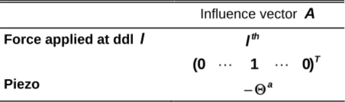
A is the influence vector of the actuator, depending of the actuator type (see table II).
TABLE II. INFLUENCE ACTUATOR VECTOR Influence vector A Force applied at ddl l T th l ) 0 1 0 ( Piezo −Θa
THEORY OF PRINCIPAL COMPONENT ANALYSIS
The summation given in (5) shows that, for limited frequency bandwidth (e.g., by means of anti-aliasing filters required for data sampling), the piezoelectric sensor responses are constrained to lay in a subspace generated by the lower structural modes and the residue of higher frequency modes:
( )
( )
( )
s r r m i i s i T T t t t q =∑ Θ Φ + Θ Φ =1α α (6)where Φr is the global residue of the higher frequency modes.
This important fact suggests that the subspace covered by the structural responses is independent of the history of the excitation, at least for broadband frequency spectrum.
Computation of the Principal Component Subspace using SVD
In fact, it is not necessary to identify the dynamic modes if we are able to compare the response subspaces between the initial and damaged states. The singular value decomposition (SVD), which is related to the PCA, is a powerfully useful and straightforward approach to compute a modal metrics of test data. This paper assumes that the number of sensor M is greater than the number of involved structural modes m+1 in order to assure a redundancy of data (e.g., M≥ m+2). Let q(t) denote a discrete block time-history, where q is a vector containing the b sampled responses of the M
piezoelectric sensors (generally, b>>M):
( )
( )
( )
( )
⎥⎥ ⎥ ⎦ ⎤ ⎢ ⎢ ⎢ ⎣ ⎡ = + + + + b j M j M b j j t q t q t q t q Q 1 1 1 1 (7)the SVD of the block data Q gives:
T
V U
Q= Σ (8)
U is an orthonormal matrix (MxM) where the columns lay a geometrical subspace generated by the sensors. Each columns of U are associated with the time factors V (NxN), and with singular values sorted in descending order, given by the main diagonal of Σ (Mxb). The singular values of Q can be interpreted as the energy associated with the principal components of U; this means that the structure will react mainly to the directions of the principal components associated with the highest energies. If we are only interested in the subspace of the responses, it will be computationally more efficient to calculate the SVD of:
T
T U U
Q
Q = Σ2 (9)
Theoretically, only the first m+1 eigenvalues of Q are non-zeros. Nevertheless, we know that test data contains redundant, linearly dependent information and also noise. Sensor noise in the test data will place constraints on the conditioning which are much more stringent than encountered in purely analytical problems. Hopefully, since noise has much lower energy than the structural modes, its effect will be easily detected and discarded from the principal component subspace. In practice, components of U associated with eigenvalues presenting an order of magnitude much lower than others has to be discarded of the principal component base.
Angles between Subspaces
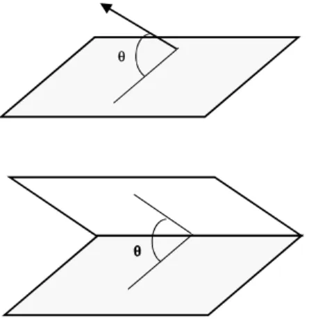
One way to compare subspace is to use the concept of angle between two subspaces. In three dimensions, it is easy to visualise the angle between one vector and one plane or between two planes (see figure 1). This method is then able to quantify the spatial coherence between two time-history blocks of an oscillating system.
θ
Figure 1. 3-D geometrical interpretation of the concept of angle between subspaces
Golub et al. [7] describe the concept and the computation of angle between subspaces. Let A∈ℜMxp and B∈ℜMxq
(
p≥q)
each with linearly independentcolumns, there will be q principal angles between the subspaces spanned by A and B. These principal angles are computed by first applying a QR factorisation on A and B, the columns of QA and QB will then define
orthonormal bases of A and B respectively:
Mxq B B B Mxp A A A Q R Q B Q R Q A ℜ ∈ = ℜ ∈ = (10) The singular values of QTAQB compute the q cosines of the principal angles
i
θ between A and B:
(
Q Q)
diag(
( )
)
i qSVD TA B ⎯⎯→ cosθi =1… (11)
The largest angle quantifies then how the subspaces A and B are globally different.
Detection of the damaged sensor
As already mentioned in the introduction, [5] gives the general principle for the detection of a damaged sensor by considering the subspace of the response compared to the subspace generated by the lower modes (assumed known with accuracy) of the structure. The idea of this paper is to rather compare response subspaces between initial and current states.
The problem is reduced to identify which sensor set affects the sensor subspace. Sensors are then split into two groups: those assumed damaged and those assumed undamaged. By remembering that small damages do not affect significantly the structural dynamics but affect directly the response of the involved sensor, the undamaged sensor subspace will not exhibit appreciable differences between initial and damaged states. Of course, we do not know which sensors are damaged and, therefore, each potential subset of sensors should be tested. Practically, the identification of one damaged sensor is performed by measuring the maximum subspace angle between the pre- and post-damaged states and by successively taking out each lamina from the sensor set; the maximum subspace angle will be minimum when the damaged lamina is discarded from the working sensor subset.
NUMERICAL EXAMPLE
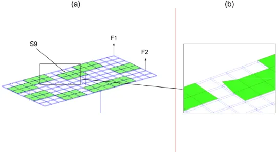
The method for damage detection, presented in this paper, has been applied on a numerical example. The main structure consists of an 0.16 x 0.08 x 0.001 m stainless steel plate, fixed in 3 points (see figure 2(a)) and fitted with 9 PZT-lamina sensors (0.003 x 0.002 x 0.000254 m), assumed connected to charge amplifiers. The tested structure is modelled using the
(a) (b)
Figure 2. Structural finite element model (a) with damage details (b)
finite element technique. The model uses conventional 3-D isoparametric solid elements, improved by adding incompatible second order shape functions associated to node-less degrees of freedom. This technique has been introduced by Bathe and Wilson [9] and applied to piezoelectric structure by Tzou and Tseng [10]. The structure presents 5 modes in the band of frequencies [0-600 Hz] (see table 3). Modal damping of 0.5% is
F1
F2 S9
included. Randomly distributed noise with amplitude of 1% of the maximum responses is added to each sensor. Responses are sampled in 1024 equally spaced time within a frequency band of [0-600 Hz].
TABLE III. STRUCTURAL RESONANCE FREQUENCIES
Undamaged 1/12 damaged 3/12 damaged
137.7 Hz 137.6 Hz 136.8 Hz
171.0 Hz 170.7 Hz 169.9 Hz
465.9 Hz 464.7 Hz 461.8 Hz
478.8 Hz 478.7 Hz 478.5 Hz
582.1 Hz 581.8 Hz 581.0 Hz
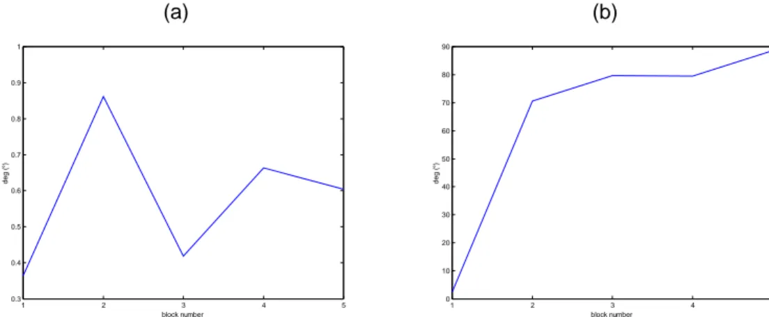
Figure 3(a) compares, at 5 blocks of data, the lamina response subspace angles corresponding to two different white-noise excitations, the structure being excited at one point labelled F1 on figure 2. This confirms that the subspace covered by the structural responses is independent of the history of the excitations. The response subspaces between a white-noise random excitation and an impact excitation at F2 (figures 4(a) and 4(b) respectively) are also compared in figure 3(b). The time-dependent decreasing correlation between subspaces is explained by the increasing influence of noise along with the time.
(a) 1 2 3 4 5 0.3 0.4 0.5 0.6 0.7 0.8 0.9 1 block number deg ( °) (b) 1 2 3 4 5 0 10 20 30 40 50 60 70 80 90 block number deg ( °)
Figure 3. Influence of excitation positions (a) and excitation shapes on subspace angles (b)
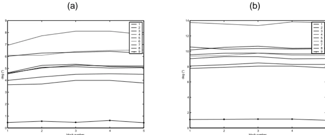
A local de-lamination on sensor 9 (see details in figure 2(b)) has been introduced for two damage levels: delaminated / healthy sensor surface ratio of 1/12 and 3/12. Non-linear effects associated with damage are neglected. Table 3 gives the first structural resonance frequencies between the different damage levels and shows that delaminations have a negligible influence in terms of modal data. Figures 5(a) and 5(b) present the
identification of the damaged lamina, by measuring the subspace angles between the pre- and post-damaged states and by testing each potential subsets of working sensors. In these two figures, it appears that subspace angle is minimum when sensor 9 is discarded from the working sensor subset. (a) 0 0.2 0.4 0.6 0.8 1 1.2 1.4 1.6 -2 -1.5 -1 -0.5 0 0.5 1 1.5 2x 10 -5 s C (b) 0 0.2 0.4 0.6 0.8 1 1.2 1.4 1.6 -8 -6 -4 -2 0 2 4 6x 10 -5 s C
Figure 4. Piezo lamina responses, structure subject to white noise (a) and impact (b) excitations (a) 1 2 3 4 5 0 1 2 3 4 5 6 7 8 9 block number deg ( °) 1 2 3 4 5 6 7 8 9 (b) 1 2 3 4 5 0 2 4 6 8 10 12 14 block number deg ( °) 1 2 3 4 5 6 7 8 9
Figure 5. Subspace angle comparisons between initial and damage states: 1/12 (a) and 3/12 (b) of damage on sensor 9
CONCLUSIONS
This paper outlines the use of piezoelectric laminas as sensor for the localisation of low amplitude structural damages. This method does not require the knowledge of neither the structural excitations nor a structural model. A strategically positioned lamina, at a zone with high probability of failure, has the ability to 'catch' damages: a local de-lamination (or an electrode deterioration) at the sensor level will then show significant changes on the sensor response. Using the concept of angle between subspaces, the problem is reduced to identify which sensor set affects the
subspace covered by the sensor responses. Sensors are then split into two groups: those assumed damaged and those assumed undamaged, each potential subset of sensors being tested.
This method gives good results and is able to detect very small damages such as a local de-lamination that would not be detected using methods based on modal data changes. Moreover, this method presents a quiet cheap computational cost and, therefore, seems adapted for the monitoring of structures with, e.g. a large number of embedded sensors. Nevertheless, it is important to point out that the thermal sensitivity of piezoelectric laminas could be a major drawback if thermal compensation is not applied.
ACKNOWLEDGEMENT
This work is supported by a grant from the Walloon government as a part of the convention n°9613500 "Identification des paramètres de couplage piézoélectrique".
REFERENCES
1. Lee, C.-K. 1992 Piezoelectric Laminates: Theory and Experiments for Distributed Sensors and Actuators, in Intelligent Structural Systems, Eds. Tzou and Anderson.
Boston: Kluwer Academic Publishers, pp. 75-167
2. Kabeya, K., Jiang, Z., Cudney H. H. 1998. “Structural Health Monitoring by Impedance
and Wave Propagation Measurement,” presented at 4th International Conference on Motion and Vibration Control (MOVIC98), Zurich, Augustus 1998.
3. Friswell, M. I. and Penny, J. E. T. 1997. “Is Damage Location using Vibration
Measurements Practical?” presented at DAMAS 97, Structural Damage Assessment using Advanced Signal Processing Procedures, Sheffield, June/July 1997.
4. Lenaerts, V., Kershen, G., Golinval, J.-C. 2001. “Proper Orthogonal Decomposition for Model Updating of Non-Linear Mechanical Systems," Mechanical Systems and Signal
Processing, 15(1): 31-43.
5. Friswell, M. I. and Inman, D. J. 2000. “Sensor Validation for Smart Structures,”
presented at the 18th International Modal Analysis Conference (IMAC-XVIII), San Antonio, February 2000.
6. Saunders, R. S., Cole, D. G., Robertshaw, H. H. 1994. “Experiments in Piezostructure Modal Analysis for MIMO Feedback Control," Smart Mater. Struct., 3: 210-218.
7. Golub, G. H., Van Loan, C. F. 1996. Matrix Computations. Baltimore, The Johns Hopkins University Press, pp. 603-604.
8. Géradin, M. and Rixen, D. 1994. Mechanical Vibrations: Theory and Application to
Structural Dynamics. Chichester, John Wiley & Sons, Ltd., pp. 52-54.
9. Bathe, K.J., Wilson, E.L. 1976. Numerical methods in finite element analysis, Englewood Cliffs, NJ : Prentice Hall
10. Tzou, H.S., Tseng, C.I. 1991. "Distributed vibration control and identification of coupled elastic/piezoelectric systems : finite element formulation and applications," Mechanical