Polarimetric active imaging : a feasibility demonstration in the infrared bands

YANNICK RASMUSSEN

POLARIMETRIC ACTIVE IMAGING

A teasibility démonstration in the infrared bands

Mémoire présenté

à la Faculté des études supérieures de l'Université Laval dans le cadre du programme de Maîtrise en physique pour l'obtention du grade de Maître es sciences (M.Se.)

DEPARTMENT DE PHYSIQUE, GENIE PHYSIQUE ET OPTIQUE FACULTE DES SCIENCES ET DE GÉNIE

UNIVERSITE LAVAL QUEBEC

2007

Résumé

Plusieurs générations de systèmes d'imagerie active aéroportés et terrestres (ALBEDOS, ELVISS, LASSIE) ont été développées et testées avec succès au centre de Recherche et Développement pour la Défense du Canada (RDDC) Valcartier [1]. Ces systèmes utilisent un illuminateur composé de puissantes diodes laser puisées fonctionnant dans la bande du proche-infrarouge et une caméra à faible niveau d'intensité (LLLTV) avec crénelage en distance.

Une technique appelée l'imagerie active par polarisation est une manière différente d'exploiter les propriétés des systèmes actifs. Cette technique emploie la polarisation de la lumière d'cclairement pour distinguer et augmenter le contraste des objets d'intérêt dans une scène. Pour appliquer cette technique, une source lumineuse polarisée fut employée et l'état de polarisation de la lumière réfléchie par la scène analysé. L'avantage avec cette méthode est que quelques objets synthétiques ou faits par l'Homme (par exemple les véhicules) réfléchissent la lumière sans changer la polarisation incidente et que les fonds naturels (par exemple l'herbe) tendent à dépolariser la lumière incidente [2-4]. Par conséquent, en analysant l'état de polarisation de la lumière réfléchie, il est possible d'augmenter le contraste des objets visés par rapport à leur arrière plan. Cette technique, également appelée discrimination de cibles par polarisation, est connue depuis un certain temps et est déjà utilisée dans des dispositifs d'imagerie passive comme les imageurs thermiques [5]. Cependant, l'application de ce concept à l'imagerie active devait être explorée et démontrée.

La technique d'imagerie active par polarisation a donc été testée dans les trois principales sections de la radiation infrarouge: 1) le proche infrarouge (>.~810 nm), 2) l'infrarouge moyen (^.~3-5 u,m) et 3) l'infrarouge lointain (À.-8-12 um). Pour chacune des ces régions, une source laser, des polariseurs et une caméra furent utilisés pour faire de l'imagerie active polarisée. Plusieurs essais en laboratoire et à l'extérieur ont été faits pour comparer cette technique avec l'imagerie passive et l'imagerie active. Ces essais ont permis de démontrer que la polarisation et le traitement de ces images augmente le contraste de la majorité des cibles étudiées par rapport au contraste obtenu avec l'imagerie active conventionnelle.

Abstract

Sevcral générations (ALBEDOS, ELV1SS, LASSIE) of airbornc and land-bascd active imaging Systems havc bcen developed and tested succcssfully at the Defence Research and Development Canada (DRDC) Valcartier [1]. They were based on a powcrful pulscd laser diode array illuminator opcrating in the near-infrared band and a range-gated low-light levcl TV (LLLTV) caméra.

A technique callcd polarimetric active imaging is a différent way to exploit the properties of active imaging Systems. This technique uses the polarization of the illuminating light to discriminatc and enhanec the contrast of objects of interest within a scène. To apply this technique, a polarizcd light source was used and the polarization statc of the light reflected by the scène was analyzed. The advantage with this method is that somc man-made objects (e.g. vehiclcs) reflect light without changing the incident polarization and that natural backgrounds (e.g. grass) tend to depolarize the incident light [2-4]. Therefore, by analyzing the polarization state of the reflected light, it is possible to enhanec the contrast of targeted objects with respect to the background. This concept also callcd targct discrimination by polarization is known for somc timc and is alrcady used in passive imaging deviecs like thermal imagers [5]. In active imaging, the application of the concept had to be explorcd and demonstrated.

Therefore, the polarimetric active imaging technique was tested for the three major bands of the infrared radiation: 1) the near-infrared (^.-810 nm), 2) the mid-infrared (X-3-5 um) and 3) the far-infrared (A.-8-12 um). For each of thèse régions, a laser source, polarizers and one caméra were used to evaluate the potential of polarimetric active imaging. Several field trials and experiments in laboratory were conducted to compare the polarimetric technique to passive and active imaging. Thcsc experiments permit to demonstrate that polarization and the treatment of thèse images enhanec the contrast of the majority of the studied target compared to the contrast obtained with convcntional active imaging.

Acknowledgements

I would like to thank Dr. Daniel Pomerleau, Président of Aerex Avionics Inc., and Vincent Larochelle for giving me the chance to work on that project and for their help. I also acknowledge Dr Pierre Mathieu, Dr. Georges Fournier, Dr. Hugo Lavoie, Dr. Gilles Roy and Dr. Denis Vincent for their help in the compréhension of the theory and of the phenomenon associated with this work. A kindly thanks to Dr. Tigran Galstian and Dr. Jean-Robert Simard because they were always there when 1 needed.

Furthermore, I would like to thank Messrs. Gilbert Tardif, Jean-François Charette, Albert Deslauriers, Mario Pichette, Marc Grenier, and Denis Dubé for their precious technical support. A spécial thank is directed to Mr. Luc Dubé for his help and its knowledge of the software Matlab 6.1 and to Marlène Grégoire for the administrational part of this project. Finally, I acknowledge the significant support provided by DRDC Valcartier Prototyping service and Infrastructure and Environment service, and ail those that I forgot.

Dedicated to my parents and sister, Richard, Sylvie and Mélissa, who made it feasible; to my girlfriend Annie, who made it a pleasure; to my colleagues and friends, who made itfunnier.

Contents

Résumé i Abstract ii Acknowledgements iii

Contents v List of tables vii List of figures viii Introduction 1 1 Polarization 4 1.1 Polarization 5 1.2 Jones calculus 7 1.3 Stokes calculus 9 1.4 Mueller calculus 12 1.5 Optical components 14 2 Génération of polarization 17 2.1 Absorption polarizers 17 2.2 Wire-grid polarizers 18 2.3 Polarization by reflection (Brewster angle plate) 19

2.4 Polarization by refraction (Prism polarizers) 20

2.5 Creating Circular polarization 21

3 Liquid crystals 24 3.1 History 24 3.2 Properties of liquid crystals 25

4 Light scattering 28 4.1 Dipole oscillation 28

4.2 Scattering 32 4.3 Brillouin scattering 32

4.4 Rayleigh and Mie scattering 35

4.5 Raman scattering 37 5 Molecular response to light 39

5.1 Chirality of molécules 39 5.2 Depolarization and chirality 41 5.3 Interaction of light with molécules 42 5.4 Light, molécules and their associated phenomena 45

6 Interaction of polarized light with végétation 50

6.1 Composition of leaves 50 6.2 Reflection and transmission through leaves 51

6.3 Polarization of light scattered by végétation 53

7 Scattering mathematical models 55 7.1 Scalar Kirchhoff model; reflection on rough metallic surface 55

7.2 Beckmann and Spizzichino's model 59 7.3 Specular and diffuse reflection 62 8 Radiometric model of polarimetric active imaging 65

8.2 Approximations 67 8.3 Polarization 69 8.4 Noise 70 9 Conclusions on the theoretical sections 71

10 Methodology of experiments 77

10.1 Linear polarization 77 10.2 Circular polarization 79 10.3 Images acquisition method 81

11 Near-Infrared System 83 11.1 Expérimental set-up for 805 nm opération 83

11.2 Results in laboratory 85 11.2.1 Linear polarization configuration results 87

11.2.2 Circular polarization configuration results 93

11.3 Results analysis 96 12 Characterization with an ellipsometer 100

12.1 Methodology and results 100 12.2 Depolarization values comparison 103

13 Médium wave infrared system 105 13.1 Expérimental set-up for 3.7 um opération 105

13.2 Results in laboratory 106 13.2.1 Linear polarization configuration results 108

13.2.2 Circular polarization configuration results 110

14 Far-infrared System 112 14.1 Expérimental set-up for 10.6 um opération 112

14.2 Theoretical considérations 114

Conclusion 115 Bibliography 117 Appendices 120

Annex 1: Depolarization values, ellipsometer 120 Annex 2: Depolarization values at 805 nm, ellipsometer and NIR system 121

Annex 3: Plot profiles along a horizontal line for the plant with hidden métal pièce

List of tables

Table 1. Stokes vectors for some typical polarization states where 0 is the angle between the horizontal (x axis) and the electric field vector. Table reproduced from Huard [11].

11 Table 2. Jones and Mueller matrices for some of the most important optical components.

Table extracted from Saleh and Teich [9] and Huard [11] 15 Table 3. Materials and surface finishes of the targets utilized as références for the

laboratory measurements. Refer to Figure 24 86 Table 4. Simple contrast calculations (eq. 11.1) for active imagery without polarization

(Figure 25c) and for polarimetric active imaging in linear (Figure 25d) and circular

(Figure 29d) polarization 98 Table 5. The most valid depolarization values ((3) for the targets (plates) used for the

laboratory expérimentations measured with the University Laval's ellipsometer, from

700 to 1700 nm 102 Table 6. Some depolarization values for target (plates) used for the laboratory

measurements. Comparison of the values taken at 805 nm with the University Laval's ellipsometer and values acquired with the polarimetric NIR active imaging System for

both linear and circular polarizations 104 Table 7. Depolarization values for each target (plates) used for the laboratory

measurements, complementary to Table 5. Values taken with the University Laval's

ellipsometer, from 700 to 1700 nm 120 Table 8. Depolarization values for each target (plates) used for the laboratory

measurements. Comparison between values from the ellipsometer and from the NIR

List of figures

Figure 1. Time course of the electric field vector at several positions: (a) arbitrary wave;

(b) paraxial wave or plane wave traveling in the z direction. Figure drawings based on

Saleh and Teich [9] 4

Figure 2. a) Rotation of the endpoint of the electric-field vector in thex-y plane at a fixed

position z. b) Snapshot of the trajectory of the tip of the electric-field vector at time t.

Figure drawings based on Saleh and Teich [9] 6

Figure 3. Picture of linearly polarized light at: a) fixed position z; b) fixed time t. Figure

drawings based on Saleh and Teich [9] 6

Figure 4. (a) Picture of right circularly polarized light and (b) left circularly polarized light

as seen by an observer "receiving" the light. Figure drawing based on Saleh and Teich

[9] 7

Figure 5. Jones vectors for some spécifie polarization states. Figure drawings based on

Saleh and Teich [9] 9

Figure 6. Représentation of the Poincaré sphère. Figure drawing based on Huard [11],

Brosseau [12] and Jerrard [13] , 11

Figure 7. Dual Rotating Retarder Mueller-matrix imaging polarimeter for transparent

samples. Figure drawing based on Azzam [14] 14

Figure 8. Schematic of a dual rotating retarder Mueller-matrix polarimeter for

non-transparent samples. Figure drawing based on Azzam [14] 14

Figure 9. Some of the poiarizing beamsplitter: a) Rochon prism, b) Wollaston prism and c)

Glan-Thompson (isotropic glue) or Glan-Foucault (air) prism. Figure drawn from

Saleh and Teich [9] 21

Figure 10. How a Fresnel rhomb can create circularly polarized light. Figure drawn from

Huard [11] 23

Figure 11. Orientation of the molécules in the three main types or phases of liquid crystals:

a) Nematic, b) Smectic and c) Cholesteric. Figure drawings based on Saleh and Teich

[9] and Jacobs et al. [15] 26

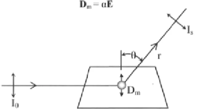
Figure 12. Linearly polarized plane wave of intensity lo incident on the molécule induces a

dipole moment Dm. The oscillating dipole produces radiation of intensity Is at distance

r and angle 0 29

Figure 13. Approximate wavelength shifts of the scattered light depending on which

phenomenon is occurring 32

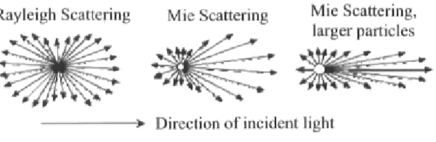
Figure 14. Comparison for Rayleigh and Mie scattering of a light incident on particles of

différent sizes 35

Figure 15. Diagram explaining the fluorescence process 47

Figure 16. Diagram of leaf structure [25] 50 Figure 17. Transmission, réflectance and absorption of light by a leaf depending on the

wavelength [26] 52

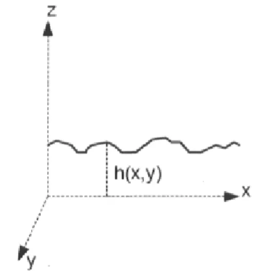
Figure 18. Angular définition of the scattering conventions 57 Figure 19. Roughness of a surface defined a distance between the rough surface and a

smooth surface 58

Figure 21. Two schematic représentations for the radiometric model: a) Point target where

the illumination footprint is bigger than the target area, therefore its scattering area is range independent; b) Extended target where the target reflects ail the incident

illumination and its scattering area is range square dépendant 65

Figure 22. Diagram explaining circular polarizer in active imaging. Figure extracted from

the Edmund Industrial Optics catalogue [36] 81

Figure 23. Ambient light color image and scheme of the System used for laboratory

measurements at 805 nm 83

Figure 24. Ambient light color image of the targets used for laboratory measurements 85 Figure 25. Linear polarization set-up (805 nm). a) Images of the targets used for laboratory

measurements with axis of transmission of both polarizers fixed in the same plane (parallel). b) The same targets, but the axis of transmission of the polarizer in front the caméra fixed perpendicular to the polarization plane of the laser (cross), c) Picture of targets in active imaging without polarization. d) Final image from the calculation of

équation 10.1 with pictures a) and b) 88

Figure 26. a) Plot of profiles along a horizontal line on row B shown in Figure 24 for

picture presented in Figure 25. Each curve corresponds to the profile of a spécifie System configuration, pictures in Figure 25. b) Plot profiles along a horizontal line

passing on every Spectralon® in pictures of Figure 25 89

Figure 27. A typical interior plant. One pièce of aluminium non-treated and one pièce of

rusted iron was partially hidden. a) Image in parallel polarization and b) in

perpendicular polarization. c) Color picture during daylight of that plant with the 2 targeted object partly hidden. d) Resulting image in polarization degree computed

using équation 10.1 91

Figure 28. a) Plot of profiles along a horizontal line on row B shown in Figure 24 for

picture presented in Figure 29. Each curve corresponds to the profile of a spécifie System configuration (see Figure 29). b) Plot of profiles along a horizontal line passing

on every Spectralon® in pictures of Figure 29 94

Figure 29. Circular polarization set-up (805 nm). a) Images of the targets used for

laboratory measurements with a left circularly polarized beam incident on the targets. b) The same targets, but a right circularly polarized beam is incident on the targets. c) Picture of targets in active imaging without polarization. d) Final image from the

calculation of équation 10.2 with pictures a) and b) 95

Figure 30. Perfect blackbodies radiation as a function of the wavelength and the

température based on Planck's law [42] 107

Figure 31. Picture of targets in passive imaging without polarization (3-5 um) 107 Figure 32. Linear polarization set-up in the MWIR band (3.7 um). a) Images of the targets

used for laboratory measurements with axis of transmission of both polarizers fixed in the same plane (parallel). b) The same targets, but the axis of transmission of the polarizer in front the caméra fixed perpendicular to the polarization plane of the laser (cross), c) Picture of targets in active imaging without polarization (3.7 um laser), d)

Final image from the calculation of équation 10.1 with pictures a) and b) 109

Figure 33. Circular polarization set-up in the MWIR band (3.7 um). a) Images of the

targets used for laboratory measurements with a left circularly polarized beam incident on the targets. b) The same targets, but a right circularly polarized beam is incident on

the targets. c) Picture of targets in active imaging without polarization (3.7 um laser).

d) Final image from the calculation of équation 10.1 with pictures a) and b) 111

Figure 34. 3-D représentation in Solid Edge® VI8 of the Far-IR polarimetric active

imaging System 113

Introduction

The use of electro-optical instruments and sensors in military opérations has been increasing rapidly in récent years. The overwhelming advantages enjoyed by a force that owns devices like laser rangefinders, designators, night-vision goggles, day and night caméras and thermal imagers were évident during the last conflicts (90-91 Gulf war, Kosovo, Afghanistan, Iraq), when the (US-led) various coalitions made extensive use of thèse technologies. During conflicts or peacekeeping missions in which the Canadian Forces hâve participated, the short-to-medium range capabilities of thèse optronic devices and their complementary rôle to radar were appreciated. Radars are well-known long-range, all-weather détection sensors, with generally poor resolution, as optronic sensors are shorter range, high-spatial resolution imaging devices. Today, almost ail surveillance platforms are equipped with some electro-optical (EO) sensors and, in the near future, it is expected that active imaging Systems presently under development will be added to this list.

Active imagers are capable of detecting and identifying targets in complète darkness and, to some extent, in adverse weather conditions. They overcome several deficiencies encountered with common CCD caméras, image intensified Systems and thermal imaging sensors. The technique consists in illuminating a scène with an artificial light source and detecting the reflected or backscattered photons. Contrary to passive imaging Systems which rely on either the reflected light from the background radiation or the thermal emitted radiation of objects in the scène, active Systems use their own source of illumination and are therefore less sensitive to the ambient light conditions to the point of being able to operate in complète darkness. The range gating mode isolâtes the target from the background and excludes the effects of light backscattering that arises from haze, snow or rain présent in the sensor's fïeld of view. Also, in some cases, it reduces significantly the blooming effect caused by the présence of bright lights as often encountered when using NVGs. Finally, NIR active Systems can image through windshields vehicle interiors at night, detect at long ranges optical sights (cat's eye effect) and gather at night target évidences like lettering. One important feature of active imagers is that the operator can sélect or control the various parameters of illumination like the active field of view, the

position and depth of the intensified range and, the laser wavelength, energy, puise width and répétition rate.

The Advanced Surveillance Sensors Group at the Defence Research and Development Canada (DRDC) Valcartier has the mandate to explore new surveillance sensor concepts to enhance détection, récognition and identification of maritime, surface or airborne targets. One of the Group's axes of research is to investigate new imaging technologies to improve Canadian Forces surveillance and reconnaissance capabilities.

Polarization is also an important property of light and represents a fundamental concept in several technological fields such as imagery, télécommunication, medicine and instrumentation. Many applications use active cohérent illumination and analyze the variation of the polarization state of the optical signal [6]. Polarization of light has been used and studied by many people in the past for différent applications [7]. The présent document investigates the target contrast enhancement obtained by using a polarized laser source in an active imager and by analyzing the polarization of the reflected light. This technique is known as polarimetric active imaging and is based on the discrimination property that man-made objects will not depolarize light as much as natural background will [2-4, 8]. This technique has a strong potential to be a powerful method for detecting objects that hâve a low contrast in classical intensity images. The complexity of this subject requires an overview of the majority of the topics related to the effects of nature on polarization. Consequently, one should know and understand the polarization phenomena taking place when analyzing images acquired in polarimetric active imaging. This will permit a better understanding of the resulting images and/or allow an estimation of the results before acquiring any images.

This document starts with the introduction of the various polarization modeling concepts (Jones, Stokes and Mueller matrices or vectors) that represent the light beam, the optical éléments and their interaction. Then, a brief review of the major polarization components is done. A small study on light scattering (molécules, végétation and surfaces) with a polarization considération is expressed and a radiometric model to anticipate the returned

signal from a scène is developed. The main conclusions on this reviewing are then presented. The methodology of experiments follows, expérimental set-ups are described and laboratory measurements carried out in the near-infrared médium wave infrared on selected targets of various materials and surface conditions are presented. Finally, a prototype for a polarimetric active imager in the LWIR spectral band is introduced. Thèse Systems hâve demonstrated that this technique exhibits some potential and interesting exploitable properties.

1 Polarization

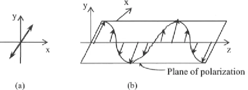
The polarization of light is, in someway, an obscure property because it is not directly détectable by the human eye (this isn't true for ail animais—bées for example reportedly navigate by the polarization of sunlight scattered by the atmosphère.). The polarization of light is determined by the time course of the direction of the electric-field vector £?(r,t). For monochromatic light, the three spatial components of £(r,t) vary following sinusoidal functions with time as it propagates through space. In gênerai, monochromatic waves hâve amplitudes and phases that are différent, so that for each position r, the endpoint of the vector <?(r,t) moves and traces in a plane an ellipse as illustrated in Figure 1. The plane, the orientation, and the shape of the ellipse generally vary with position.

(a) (b)

Figure 1. Time course of the electric field vector at several positions: (a) arbitrary wave; (b) paraxial wave or

plane wave traveling in the z direction. Figure drawings based on Saleh and Teich [9].

However, in paraxial optics, light propagates along directions that lie within a narrow cône centred on the optical axis (the z axis). Waves are approximately transverse electromagnetic (TEM) where the electric-field vector lies approximately in the transverse plane (the x-y plane) as illustrated in Figure 1. If the médium is isotropic, the polarization ellipse is approximately the same everywhere and the wave is said to be elliptically

polarized. The orientation and eccentricity of the ellipse détermine the state of polarization

of the optical wave, whereas the size of the ellipse is related to the optical intensity. When

the ellipse dégénérâtes into a straight line or becomes a circle, the wave is said to be

linearly or circularly polar ized, respectively.

1.1 Polarization

Considering a monochromatic wave of frequency v traveling in the z direction with velocity c, the electric field lies in the x-y plane and is generally described by:

e(z,i) - R e - ^ e x p 2J7TV f z^ t — (î.i)

where the complex envelope A=Axx + Ayj> is a vector with complex components Ax and Ay. To define the polarization ellipse, we express Ax and Ay in terms of their respective magnitude and phase, Ax = ax exp(j^) and Ay = ay exp(j<pr). Substituting into (1.1), we obtain: £(z,t) - exx+ ey y where ex = ax cos 2nv t—

A

A

are the x and y components of the electric-field vector e(z,t). The components ex and ey are periodic functions of t - z/c oscillating at frequency v. Manipulating mathematically équations (1.3) and (1.4), it is easy to show that thèse équations are the parametric équations of the ellipse [10]

^ - + —j- - 2 cos ç = sin 2<p ,

a. a., a,.a„

(1.5)

(a) (b)

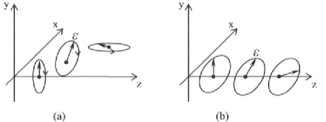
Figure 2. a) Rotation of the endpoint of the electric-field vector in the x-y plane at a fixed position z. b)

Snapshot of the trajectory of the tip of the electric-field vector at time t. Figure drawings based on Saleh and Teich [9].

At a fixed value of z, the tip of the electric-field vector rotâtes periodically in the x-y plane, tracing out an ellipse. At a fixed time t, the locus of the tip of the electric-field vector follows a helical trajectory in space lying on the surface of an elliptical cylinder (see Figure 2). The shape of the ellipse détermines the polarization state of the wave.

If one of the two components of équation 1.5 vanishes (e.g. ax=0), the light is linearly

polarized in the direction of the other component (the y direction in the current example).

The wave is also linearly polarized if the phase différence cp - 0 or n, or if ax - ay (see

Figure 3).

Plane of polarization

(a) (b)

Figure 3. Picture of linearly polarized light at: a) fixed position z; b) fixed time t. Figure drawings based on

Saleh and Teich [9].

If <p = ±n/2 and ax = av = a0, équation (1.5) becomes e] + s2y = a^which is the équation

of a circle, so the wave is said to be circularly polarized. If <p = - n/2, the electric field at a fixed position z rotâtes in a clockwise direction when viewed by an observer receiving the

wave, so the light is right circularly polarized. The case (p = + n/2 corresponds to counter clockwise rotation and the light is said to be left circularly polarized (see Figure 4).

y A

(a) (b)

Figure 4. (a) Picture of right circularly polarized light and (b) left circularly polarized light as seen by an

observer "receiving" the light. Figure drawing based on Saleh and Teich [9].

1.2 Jones calculus

As shown previously, the complex envelope A=Axx+Ayy of a monochromatic plane wave

is a vector where its complex components are expressed as Ax = ax exp(j<^) and Ay = ay

exp(j#>,,). It is convenient to write thèse complex quantities in the form of a column matrix:

J = (1.6)

This column matrix is called Jones vector. With this vector, we can détermine the total intensity of the wave defined as / = (|^|2 + L4v\2)/2rj, rçbeing the refractive index of the

médium in which the wave propagates. Furthermore, we use the ratio ax/av = \AX\/\A\

and the phase différence ç = (pY-(px - arg\Ay)-arg{Ax} to détermine the orientation and

shape of the polarization ellipse [9-11].

The Jones vectors, for some spécial polarization states, are shown in Figure 5. The intensity for each case has been normalized so that \AX\2 + \Ay r = 1 and the phase of the x component

Now, consider the transmission of a plane wave of arbitrary polarization through an optical System that maintains the plane-wave nature of this wave, but changes its polarization. The System is assumed to be linear, so that the principle of superposition of optical fields applies. The complex envelopes of the two electric-field components of the incident wave,

Alx and A[v, and those of the transmitted or reflected wave, A2x and A2y are in gênerai

related by the following weighted linear combinations:

Ajx - T\\AU +Ti2A[y

Ajy -T2\A[x +T22Aly

(1.7) where Tu,T]2,T2i,and T22 are constants describing the optical System. Thèse linear

relations may conveniently be rewritten in a matrix notation by defining a 2x2 matrix T with éléments Tu,Tu,T2i, and T22 as follow,

■ ? i '.'.• T y ' >i 22 *\y (1.8)

The matrix T, called the Jones matrix, describes the optical System. The structure of this matrix gives its effect on the polarization state and the intensity of an incident wave. The Jones matrices for the most common optical components are shown in Table 2.

Linearly polarized wave in x direction

Linearly polarized wave, plane of polarization making angle 0 with x axis

cos# sin#

y *

y A »

Right circularly polarized wave 1 V2~ -J

Left circularly polarized wave

S

Figure 5. Jones vectors for some spécifie polarization states. Figure drawings based on Saleh and Teich [9].

1.3 Stokes calculus

In 1852, George Stokes proposed the use of a vector, which contains only four observable quantities in order to describe the polarization state of light. Thèse terms are defined experimentally and are mathematically related to the electromagnetic field. Consider a beam of light in an arbitrary state of polarization (either fully, partially, or non-polarized) analyzed by four différent types of polarizers.

First, the quantities P0,Pl,P2 and F3 are introduced to define the following quantities:

P0=A2x+A2y=Ix+Iy=Ic

P =Al-Al =1-1..

(1.9)

P2 =2AxAycos(p = I+45., -I_4S.

P3 = 2AxAysm<p = Ilefi-Irlghl

Thèse quantities are called the Stokes parameters. Io corresponds to the total intensity of the beam, Ix and Iy the intensity of linear polarization of the beam along thèse axis, I+45 and L45

the intensity of linear polarization at 45 or -45 degrees compared to the x axis and finally, Iicft and Irighc is the intensity of left and right circular polarization of the beam, respectively. Thèse four parameters are not independent because they dépend on cp and on the ratio tan ^ = Ayj'Ax [11]. It's easy to show that they are related together as follow:

P2 + Pi + P32 (1.10) If we rewrite thèse parameters as 50ili2>3 = ^0,1,2,3 ^0 > '* is possible to regroup thèse ratios in

a state vector, the normalized P vector. Thèse new ratios are defined as the normalized Stokes parameters. The Poincaré sphère, conceived by Henri Poincaré around 1892 provides a convenient way of representing polarized light and predicting how any given

médium will change the polarization form. This représentation uses the normalized Stokes parameters S, ,S2 and S3 as a coordinate system. The values of thèse parameters for a light

beam represent the coordinates of a point on that sphère and a vector linking this point to the origin of the coordinate system (see Figure 6).

Now, using

S{ = cos2^ cos2«

• S2 - cos 2e sin 2a, (111)

S3 = sin 2s

any light polarization can be described by 51,52 and S-, with the Poincaré sphère. A point

M on the Poincaré sphère is defined by the vector P with its spherical coordinates

\\,2a,2e). By inspecting équation 1.11, it may be seen that this sphère has a diameter equal

to 2. Each point on that sphère corresponds to a unique state of polarization. The equatorial circle represents ail the linear states, the top of the sphère (S3 = 1, S2 = 0, Si = 0) is the

right circular polarization and the bottom (S3 = -1, S2 = 0, Si = 0) is the left circular polarization (see Figure 6). Any other point that is not situated on the equator or on the pôle of the Poincaré sphère, corresponds to an elliptic polarization state.

Partially polarized light is represented on the Poincaré sphère by an agglomération around the point (M, Figure 6) of a spécifie polarization state (elliptic, linear or circular). The smaller is this agglomération of points, the more this light can be represented as a spécifie polarization state. In the case of unpolarized light, it is considered that the light contains ail the possible states of polarization and that ail the point on the Poincaré sphère has the same likelihood.

With the parameters 5|,52 and S3 measured for a given beam, its polarization state is

determined without ambiguity. However, this représentation provides no information on the amplitude and phase of the beam. It is also important to mention that the coordinate System of the Poincaré sphère is not Cartesian (Oxyz), but refers to the Stokes parameters.

s

Right circularly polarized

Vertical (y) linearly polarized Constant Azimuth Constant Ellipticity Horizontal (x) linearly Si polarized Linear States Linearly polarized at +45° Left circularly polarized

Figure 6. Représentation of the Poincaré sphère. Figure drawing based on Huard [11], Brosseau [12] and

Jerrard[13].

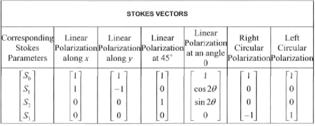
Table 1. Stokes vectors for some typical polarization states where 8 Is the angle between the horizontal (x axis) and the electhc field vector. Table reproduced from Huard [11].

STOKES VECTORS Corresponding Stokes Linear Polarization Linear Polarization Linear Polarization Linear Polarization at an angle 0 Right Circular Left Circular Parameters along x along y at45°

Linear Polarization at an angle 0 Polarization Polarization ~S0' S,

A.

T

1.4 Mueller calculus

When the polarization of light is in a pure state (totally polarized light), the Jones représentation is well adapted. But in the case of partially polarized light and for natural light, we hâve to add a cohérence matrix to use the Jones formalism. The method arising from this "addition" is called the Mueller matrix method. The description of optical Systems in terms of Mueller matrices is better adapted to gênerai cases than the Jones matrices.

The same assumptions as those made for the détermination of the Jones matrix are made hère. Considering the transmission of a plane wave of arbitrary polarization through an optical System that maintains the plane-wave nature of this wave but changes its polarization, the Mueller concept is written as

S'=MS, (1.12) where S' refers to the Stokes vector of the transmitted wave, M refers to the Mueller matrix

describing the optical device and S is the Stokes vector of the incident plane wave. Contrary to the Jones formalism, which considers the amplitudes and phases (complex numbers) of the electromagnetic field, the Stokes-Mueller formalism uses the real quadratic values (intensities along horizontal, vertical axes...) directly measured from the experiment.

Normally, the Mueller matrix of an optical device is expérimentally characterized. However, in most cases, we do not hâve to experimentally obtain this information because the Mueller matrices for the most important optical devices hâve been calculated and are given in the scientific literature. Several of thèse matrices are listed in Table 2.

In theory, a complète analysis of the polarization to détermine the Mueller matrix requires 16 measurements, which are necessary to solve the linear System containing the 16 unknown coefficients of the 4 x 4 Mueller matrix. Thèse coefficients are obtained using the Dual Rotating Retarder Technique (DRRT) introduced by Azzam [14] (see Figure 7). The

main concept with this technique is to illuminate the sample with four différent states of polarization and to analyze the transmitted light of each state.

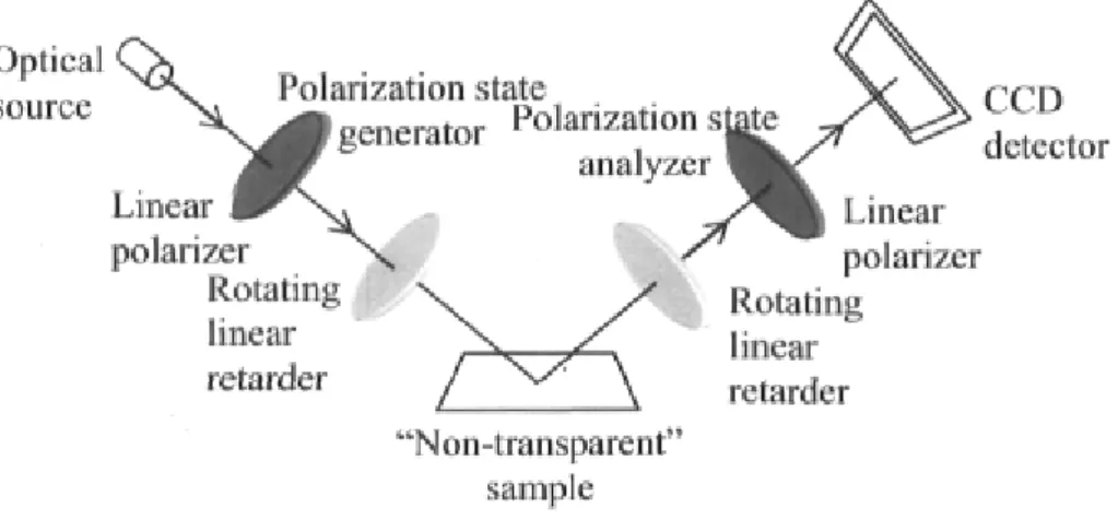
To compute the Mueller matrix with the DRRT, the optical set-up shown in Figure 7 is used. The DRRT is composed of 4 main components: l) the émission of light, 2) the polarization state generator (PSG), 3) the polarization state analyzer (PSA), and 4) the détection and signal processing. This set-up is used for "transparent" samples. In the case of "non-transparent" samples such as metals, the PSA and the detectors are re-positioned next to the PSG in such way that the backscattered light can be collected (Figure 8).

First, the PSG and PSA linear polarizers are placed in open configuration (their axes of transmission are parallel). Second, the linear retarders of PSG and PSA are fixed at the same angle position (0° for example), and a detector measures the intensity image. Turning the PSA linear retarder at four angle positions (0°, 45°, 90° and 135°), the intensity image of the polarization incident on the sample is acquired by the detector (normally a CCD caméra). Third, the linear retarder of PSG is fixed to 45°, 90° and 135° successively and the PSA linear retarder is turned at four angle positions (0°, 45°, 90° and 135°) for each angle position of the PSG linear retarder. So, an intensity image is found for each of the four angles positions of the PSG and PSA linear retarders. A total of 16 intensity images are acquired. Thèse images, measured by the CCD caméra, are the parameters of the Mueller

matrix for the sample. A computer acquires the data (16 images) and dérives two images

encoded in intensity and in polarization degree. The polarization degree Pd'is given by [5]:

Pd = \W

i

EW-M

;=o /=o

EW-M

;=o /=o

yjPf+PÏ+P?

ml

where the intensity I = Moo and where Po, Pi, P2 and P3 are the Stokes parameters measured experimentally (eq 1.9). A polarization degree Pd of 0% corresponds to a depolarizing sample and Pd =100%, to a non-depolarizing sample.

Polarization "Transparent" Polarization state generator sample state analyzer CD—>■

Optical Linear Rotating source polarizer linear

retarder

H4

Rotating Linear CCD linear polarizerdetector retarder

Figure 7. Dual Rotating Retarder Mueller-matrix imaging polarimeter for transparent samples. Figure drawing

based on Azzam [14]. Optical O s o^„^a ^ \ Polanzc source

_X^^gem

generator Polarization s CCD _detector Linear polarizer Rotating linear retarder 'Non-transparent" sample

Figure 8. Schematic of a dual rotating retarder Mueller-matrix polarimeter for non-transparent samples. Figure

drawing based on Azzam [14].

The optical source is normally a laser that is often almost linearly polarized. In this case, the linear polarizers hâve their axis of transmission fixed and a rotating linear retarder is used to change the angle of polarization.

1.5 Optical components

Some optical devices hâve the capabilities to change or transform the polarization of an incident beam, The most common optical devices are the linear and circular polarizers, the wave retarders and the polarization rotators. Table 2 shows a summary of the most common optical devices with their respective Jones and Mueller matrices.

Table 2. Jones and Mueller matrices for some of the most important optical components. Table extracted from Saleh and Teich [9] and Huard [11].

Optical

devices Jones matrix Mueller matrix

Linear polarizer along x direction 1 0 " 0 0 1 2 "1 1 0 0" 1 1 0 0 0 0 0 0 0 0 0 0 Linear polarizer along y direction 0 0" 0 1 1 ~2 1 - 1 0 0 - 1 1 0 0 0 0 0 0 0 0 0 0 Linear polarizer at 45° I 2 "1 1"

L

1

'

sin2^ cos2#sin26' sin226* 0

0 0 0 ûj Left circular polarizer 1 2 " 1 i -i 1 1 2 1 0 0 - 1 0 0 0 0 0 0 0 0 - 1 0 0 1 Right circular polarizer 1 ~2 "1 - / i 1 -, 1 2 "1 0 0 1" 0 0 0 0 0 0 0 0 1 0 0 1

Optical

devices Jones matrix Mueller matrix

Half-wave plate "1 0 " 0 - 1 " 1 0 0 0" 0 1 0 0 0 0 - 1 0 0 0 0 - 1 Quarter-wave plate "l 0~ 0 -i " 1 0 0 0" 0 1 0 0 0 0 0 1 0 0 - 1 0 Wave retarder with phase shift (p e h 0 0 e/ 2_ " 1 0 0 0 0 1 0 0 0 0 cos#> s\x\(p 0 0 -sinço cos^> Polarization rotator i -cos# - s i n # sine1 cos<9 1 1 0 0 0 0 cos2# -sin26> 0 0 sin26> cos26»0 0 0 0 0 1 16

2 Génération of polarization

A polarizer is an optical élément that is designed to produce polarized light independently of the incident light state. To do so, the polarization industry uses différent approaches and techniques. This section describes the most common techniques used to produce polarized light from unpolarized light or from others states of already polarized light.

2.1 Absorption polarizers

The absorption of light by certain anisotropic materials, called dichroic materials, dépends on the direction of the electric field and therefore dépends on the polarization of the incident light. Anisotropic materials are média where the refraction index (n) is not the same for the 3 Cartesian axes, xyz. (See section 2.4 for an explication of n0 and nc)

Uniaxial anisotropic médium Biaxial anisotropic médium nx = ny = n0 and nz = nc nx + ny + n7

When the média are absorbent, the permittivity tensor [£■] is complex, asymmetric and is not hermitic. Experimentally, this means, for example, that a polarized light will be more absorbed than another light beam having a différent polarization state. Dichroic materials hâve anisotropic molecular structure whose response is sensitive to the direction of the applied field. Sheet polarizer, operating on the principle of differential absorption along orthogonal axes, is also known as dichroic polarizer. The types of sheet polarizer typically available are molecular polarizers, i.e., they consist of transparent polymers that contain molécules, which hâve been aligned and then stained with a dichroic dye. The absorption takes place parallel the long (stretching) axis of the molécules, and the transmission axis is perpendicular to this absorption plane [10].

Polaroid is the trade name for the most commonly used dichroic material. It selectively absorbs light from one plane, typically transmitting less than 1% through a sheet of

Polaroid. It may transmit more than 80% of light in the perpendicular plane. The word "Polaroid" usually refers to Polaroid H-sheet, which is a sheet of iodine-impregnated polyvinyl alcohol. A sheet of polyvinyl alcohol is heated and stretched in one direction while softened, which has the effect of aligning the long polymeric molécules in the stretching direction. When dipped in iodine, the iodine atoms attach themselves to the aligned chains. The iodine atoms provide électrons that can move easily along the aligned chains, but not perpendicular to them. Light waves with electric fields parallel to thèse chains are strongly absorbed because of the dissipative effects of the électron motion in the chains. The direction perpendicular to the polyvinyl alcohol chains is the "transparent" direction since the électrons cannot move freely to absorb energy. Therefore, Polaroid sheet can be used to polarize a visible or near IR light beam at low cost and if the application needs a large polarizer in dimension (Polaroid sheet can be produced in several squared feet).

2.2 Wire-grid polarizers

Wire-grid polarizers consist in a planar array of parallel wires placed on a substrate. Basically, avoiding détails or mathematical models, the principle of opération of this type of polarizer is based on the diffraction of an electromagnetic wave by a periodical grating of metallic wires deposited on a substrate on refraction index n. If the period d of this grating is smaller than the wavelength of the incident light beam X, the component of the electric field E parallel to the wires is reflected and the perpendicular component is transmitted. If the métal used for the wires hâve a good electric conductivity for the wavelength of the application, the loss in transmission is very low. The electric field component of the light wave parallel to the wires drives électron in the wires, thus, generating a current within the lines that causes résistive (Joule) heating and therefore, an energy loss. However, the perpendicular component is transmitted because it has no électron to drive and hence passes through without much loss [12].

Wire-grid polarizers are similar to sheet polarizers in that the transmitted light is polarized perpendicularly to the wires (molécules for Polaroid). However, light polarized parallel to

the wires is reflected instead of being absorbed as with sheet polarizers. Normally, the light beam is directed at right incidence on the polarizer. This type of polarizer is usually used in applications where the wavelength of the beam is in the infrared band (À, > 2 um), due to the difficulty to produce smaller grid spacing.

2.3 Polarization by reflection (Brewster angle plate)

When a monochromatic plane wave traveling in médium 1 impinges the planar boundary of médium 2, reflection and refraction can occur. If the média are assumed to be linear, homogeneous, isotropic, nondispersive and nonmagnetic, reflection and refraction are governed by the SnelPs law and the Fresnel équations, respectively:

n,sin^ = n2smû2 (2.1)

r

™ = i 2T '

™

(

™ )

"

_ n2cosOx -nfcos&.

S^=-(l + ^) (2-3)

n2 COS*?, + nt cos02

where the subscript 1 and 2 refer to médium 1 or 2, n is the refraction index, 9 is the angle between the beam and the surface normal in each médium, r and t are the reflection and transmission coefficients respectively. The x-polarized mode is called the transverse electric polarization (TE), since the electric field is orthogonal to the plane of incidence. The y-polarized mode is called the transverse magnetic polarization (TM), since the magnetic field is orthogonal to the plane of incidence and the electric field is parallel to the plane of incidence.

If one traced out the plots of équation 2.3, he would see that for a typical angle, says the Brewster angle (0B), the reflection coefficient of the y-polarized mode (TM) is zéro. That

means for this angle, the TM polarization is completely transmitted (refracted). At this angle, only the TE component of the incident light is reflected, so that the dielectric of médium 2 serves as a polarizer. The Brewster angle can be calculated with:

0H = tan ' 5 t (2.4)

" i

where the n are the refractive index of each dielectric of média 1 (incident beam) and 2 (refracted beam). Brewster-angle polarizers are necessarily sensitive to incidence angle and are physically long devices because the Brewster angle can be large, especially in the infrared where materials with high indices are used. Brewster-angle polarizers are used in the infrared and ultraviolet bands because sheet and prism polarizers do not operate in thèse régions of the spectrum.

2.4 Polarization by refraction (Prism polarizers)

When light refracts at the surface of an anisotropic crystal, the two linear polarizations (TE and TM) refract at différent angles and are spatially separated. Biréfringence, also called double refraction, is the property of uniaxial anisotropic materials in which light propagates at différent velocities, depending on its direction of polarization relative to the optic axis. A wave with polarization perpendicular to the optic axis will exhibit an "ordinary" index of refraction, n0 (this is often referred to as the ordinary ray). In contrast, a wave with

polarization parallel to the optic axis exhibits an "extraordinary" index, nc (the

extraordinary ray). The ordinary index, nD, is isotropic with respect to the direction of

propagation while the extraordinary index, nc, varies depending on the direction of

propagation with a maximum value for light traveling perpendicular to the optic axis and, of course, polarized parallel to it. The différence An = nc - n0 is also referred to the

biréfringence or the optical anisotropy.

Based on this property, biréfringent material can be used to polarize a light beam. There exists a wide variety of polarizing beamsplitter including the Foucault, the Glan-Thompson, the Rochon, the Wollaston and so on. Ail of thèse prisms use the same technique to create polarized light from unpolarized light. Two pièces of a biréfringent crystal are cemented by their hypoténuse. Usually, if the main requirement is to separate extraordinary (TE) from ordinary (TM) rays only from few degrees, thèse two pièces are stuck by their hypoténuses and only the optic axis of each pièce are fixed. For example, the

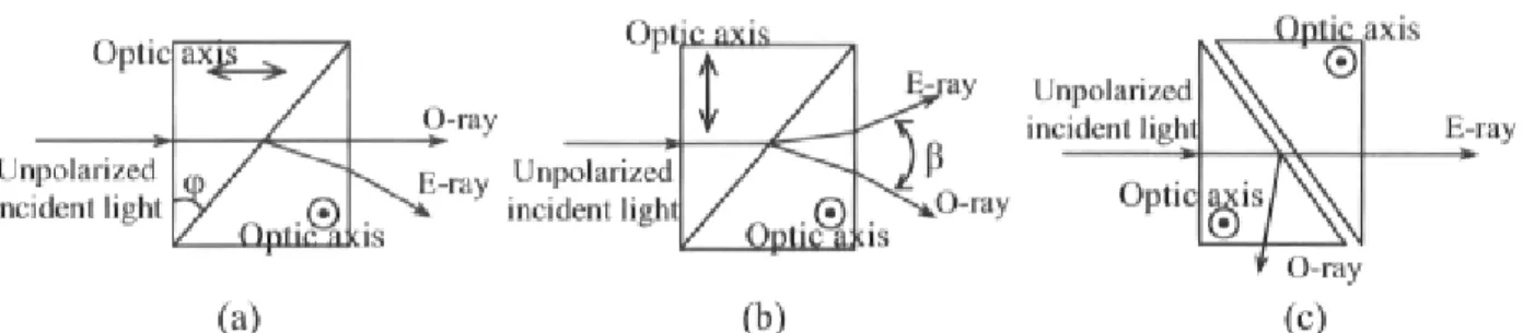
main différence between the Rochon and Wollaston prisms is how the optic axis of each pièce of the biréfringent crystal is fixed (Figure 9). The angle between the two rays (B) is dépendent on the angle of the outer wedge (p and the optical anisotropy An as

P = 2 tan '(|A/7|tan#>) (2.5)

Optic axis _{Qplic. axis}

O-ray »-Unpolarized incident light E-rav Uipolmù-œd incident light (a)

Figure 9. Some of the polarizing beamsplitter: a) Rochon prism, b) Wollaston prism and c) Glan-Thompson

(isotropic glue) or Glan-Foucault (air) prism. Figure drawn from Saleh and Teich [9].

where E-ray and O-ray refer to the extraordinary and ordinary ray, respectively. There exist no gênerai rules to know if the rays are TE or TM polarized. One should read the book of Saleh and Teich [9] or Huard [11] to see weather the rays are TE or TM polarized. The optical axis direction is oriented parallel (J or <-*) or perpendicular ( © ) to the page.

The cernent used to stick thèse pièces can be a stacking of thin layers of différent indices and thicknesses, as in the MacNeille prism, where a judicious choice for the layer permits to separate totally (about 90°) the two polarizations. Polarizing beamsplitter cubes are almost always used in the visible or near IR part of the spectrum because they hâve a high polarization resolution and a good transmission for thèse wavelengths. The industry normally uses as biréfringent crystal: quartz, calcite or Mica. One should note that the angle of séparation between both polarization increases when the wavelength decreases, because the refraction indexes change when the wavelength change.

2.5 Creating Circular polarization

In sections 2.1 to 2.4 inclusively, only components that create linear polarization from an unpolarized incident light beam are presented. However, circular polarization is also

frequently used in research. There exist two main manners to create circularly polarized light from linearly polarized light: the quarter-wave plate and the Fresnel Rhomb.

A quarter-wave plate is a wave retarder which introduces a phase retardation of 7t/2 to the incident light beam corresponding to an optical path equal to a quarter of wavelength (A/4). It is made of an anisotropic (biréfringent) material and the phase retardation (8) introduced by a wave plate is proportional to the biréfringence of the crystal:

gs2*L{nt-n0) ( 2 5)

A

where L is the thickness of the plate, X the wavelength, nc and n0 the extraordinary and

ordinary index, respectively. Therefore, when the wavelength, the indices and the desired retardation are known, quarter-wave plate is easily designed.

Thèse quarter-wave plates hâve a fast axis and a slow axis. When a linearly polarized light beam is incident on this type of retarder, with the plane of polarization exactly at 45° compared to the fast axis of the wave plate, the output beam is left circularly polarized when regarding toward the direction of the traveling beam. Based on the same phenomenon, if the plane of polarization is exactly at -45° compared to the fast axis of the wave plate, a right circularly polarized light beam will be created. One can also use a half-wave plate to create right circularly polarized light from left circularly polarized light. A half-wave plate introduces a phase retardation of n to the incident light beam. Note that the process with the quarter-wave plate is réversible. This means that if a left circularly polarized light beam is incident on such a plate, linearly polarized light with the plane of polarization at 45° compared to the fast axis will be produced.

The Fresnel Rhomb was developed in 1817 by Augustin Jean Fresnel (1788-1827) to produce circularly polarized light (Figure 10). This polarization component is normally made of glass, fused silica or BK7. A linearly polarized wave whose direction of polarization is at an angle of 45° with respect of the face edge of the rhomb of glass is normally incident on one face. The light beam in the Fresnel rhomb undergoes two total internai reflections before emerging from the exit face, resulting in a quarter-wavelength

optical path différence and a phase différence introduced between the TE and TM components of the reflected wave. Thus, as for the quarter-wave plate, the emerging light beam is circularly polarized.

Linearly polarized input light beam at 45

Left circularly polarized output light beam

Figure 10. How a Fresnel rhomb can create circularly polarized light. Figure drawn from Huard [11].

In addition, as in the case of the quarterwave plate, if the input light beam is polarized at -45° with respect of the face edge of the rhomb, the output light beam will be right circularly polarized. The angle of apex 6 of the rhomb dépends on the refraction index of the glass. For example, if the glass is made of borosilicate, refraction index n = 1.511, the apex angle should be 0 = 54°43'. This apex angle can be calculated using équation 2.6, with A = cpiE -cpiM, the différence in relative phase change between TM and TE waves. Note that to be circularly polarized, a wave must hâve A = re/4.

tan A/2 = cosOylsm20-n 2 sin26>

(2.6)

The Fresnel rhomb is normally used in the visible or near IR spectral band because of the fabrication material (glass). However, the component is bigger in dimension than a quarter-wave plate and the output beam is not aligned to the input beam. Also, if one uses two identical Fresnel rhomb in a row, this association acts as a half-wave plate because it corresponds to an optical path equal to a half of wavelength (A/2), and the output beam will be linearly polarized at -45° using a 45° polarized input light beam.

3 Liquid crystals

3.1 History

In 1888, the Austrian chemist Friedrich Reinitzer, working for the Institute of Plant Physiology at the University of Prague, discovered a strange phenomenon. Reinitzer was conducting experiments on a cholesterol-based substance trying to figure out the correct formula and molecular weight of cholestérol. When he tried to precisely détermine the melting point, which is an important indicator of the purity of a substance, he was struck by the fact that this substance seemed to hâve two melting points. At 145.5°C the solid crystal melted into a cloudy liquid, which existed until 178.5°C where the cloudiness suddenly disappeared, giving way to a clear transparent liquid. At first Reinitzer thought that this might be a sign of impurities in the material, but further purification did not bring any changes to this behaviour.

Puzzled by his discovery, Reinitzer turned for help to the German physicist Otto Lehmann, who was an expert in crystal optics. Lehmann became convinced that the cloudy liquid had a unique kind of order. In contrast, the transparent liquid at higher température had the characteristic disordered state of ail common liquids. Eventually he realized that the cloudy liquid was a new state of matter and coined the name "liquid crystal," illustrating that it was something between a liquid and a solid, sharing important properties of both. In a normal liquid the properties are isotropic, i.e. the same in ail directions. In a liquid crystal they are not; they strongly dépend on direction even if the substance itself is fluid.

The scientific community challenged this new idea, and some scientists claimed that the newly discovered state probably was just a mixture of solid and liquid components. However, between 1910 and 1930, conclusive experiments and early théories supported the liquid crystal concept at the same time that new types of liquid crystalline states of order were discovered. At the early time of Reinitzer and Lehmann, scientists only knew three states of matter. The gênerai idea was that ail matter normally had one melting point, where

it turns from solid to liquid, and a boiling point where it turns from liquid to gas. Water is a good example of this view. It melts at 0°C and it boils and becomes steam at 100°C.

In the 1960s, a French theoretical physicist, Pierre-Gilles de Gennes, who had been working with magnetism and superconductivity, turned his interest to liquid crystals and soon found fascinating analogies between liquid crystals and superconductors as well as magnetic materials. His work was rewarded with the 1991 Nobel Prize in Physics. The modem development of liquid crystal science has since been deeply influenced by the work of Pierre-Gilles de Gennes.

3.2 Properties of liquid crystals

Liquid crystals hâve a state of matter in which the ellipsoid molécules hâve oriental order, like crystals, but lack positional order, like liquid. There exist three main types or phases of liquid crystals:

1 ) Nematic liquid crystals in which molécules tend to be parallel, but their positions are random.

2) Smectic liquid crystals in which molécules are parallel, but their centers are stacked in parallel layers within which they hâve random positions, so that they hâve positional order in only one dimension.

3) Cholesteric liquid crystals are a distorted form of the nematic phase in which the orientation undergoes helical rotation about an axis.

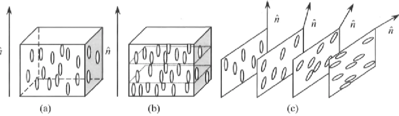
Figure 11 illustrâtes the arrangement of molécules for the three main types or phases of liquid crystals. Although the centers of gravity of the molécules hâve no long-range order as crystals do, there is order in the orientation of the molécules. They tend to be oriented parallel to a common axis which is represented by the unit vector h. The direction of h is arbitrary and is determined by some minor force such as the guiding effect of the walls of the container. There is no distinction between a positive and négative sign of h. If the molécules carry a dipole, there are equal numbers of pointing up as down. Thèse molécules

are not ferroelectric and are chiral, i.e., they hâve no handedness, and there is no positional order of the molécules within the fluid.

(a) (b) (c)

Figure 11. Orientation of the molécules in the three main types or phases of liquid crystals: a) Nematic, b)

Smectic and c) Cholesteric. Figure drawings based on Saleh and Teich [9] and Jacobs étal. [15].

Molécules in liquid crystals are bipolar and are in a fluid state of matter. Covalent bonds may resuit from atoms sharing électrons, but the sharing may not be completely equal: atoms with more protons may be able to hold their own; and other atoms borrow électrons more strongly than their partner atoms can, so that électrons spend more time around the larger atom in a covalent bond. This can create slight charge différences across whole molécules or parts of molécules - areas where électrons spend more time are slightly more négative, while areas in which they spend less time are slightly positive. Molécules with such partial charges are called polar molécules and when thèse molécules hâve only one positive side and one négative side, they are called bipolar molécules.

This particularity of the molécules (bipolarity), as in liquid crystals, permits to change the orientation of the molécules by applying a force. This force can be electrostatic, e.g. liquid crystal between two glass plates rubbed, or electric, e.g. liquid crystals between two électrodes where a voltage (electric field E) can be applied. There exists a subclass of nematic liquid crystals. Twisted nematic liquid crystals are nematic liquid crystals on which a twist, similar to the twist that exists naturally in the cholesteric phase, is imposed by external forces as described before. The twisted nematic liquid crystal is an optically inhomogeneous anisotropic médium that acts locally as a uniaxial crystal, with the optic axis parallel to the molecular direction. The optical properties are conveniently studied by

dividing the material into thin layer perpendicular to the axis of twist, each of which acts as a uniaxial crystal, with the optic axis rotating gradually in a helical manner. Twisted nematic liquid crystals hâve an orientation of the molécules ( h ), which is comparable to the one for cholesteric liquid crystals.

Under certain conditions, the twisted nematic liquid crystal acts as a polarization rotator, with the polarization plane rotating in alignment with the molecular twist. Thèse liquid crystals hâve a voltage threshold below which the polarization vector is not affected due to the internai elastic forces. The reason for this rotation is that the rotatory power of the liquid crystal is bigger that the free energy so that the electric field vector tends to aligned itself with the molécules. A dérivation of that rotatory power is given in De Vries [16] and De Gennes [17]. Considering the twist angle varying linearly with the z axis as

G = az (3.1)

where a is the twist coefficient (degrees per unit length) and the phase retardation coefficient (retardation per unit length) as

P = (n,-nX (3.2)

where nc and n0 are the extraordinary and ordinary refraction indices respectively, a liquid

crystal cell is completely described by a and p.

In gênerai, rie > n0 and (3 is much greater than a, so that many cycles of phase retardation

are introduced before the optic axis rotâtes appreciably. In addition, if the incident wave at z = 0 is linearly polarized in the x direction, then when (3 is much greater than a, the wave maintains its linearly polarized state, but the plane of polarization rotâtes in alignment with the molecular twist, as described before for twisted nematic liquid crystal. Liquid crystals find their applications in display applications, from small watch displays to large flat screen TVs and computer panels. There are many other applications in connection to information storage and handling, especially when optical solutions are sought. Liquid crystals are possible éléments to combine with others for the création of nanoscale devices. They can also be used in every application where polarization is an important factor, in medicine as much as in military applications.

4 Light scattering

4.1 Dipole oscillation

The bonding électrons are not shared equally between unlike atoms that are bonded together because of the affïnity of différent atoms in a molécule for électrons. As a resuit, the molécule may hâve a large, what is called, dipole moment. The work required to remove an électron from an isolated atom is given by the ionization potential. The tendency of an atom to pull électrons toward itself is expressed by a quantity called the electronegativity. The electronegativity of an élément, deiïned by Pauling [18], dépend on the position of that élément in the periodic table. Reading the halogen column of the periodic table from the top to the base, the atoms become less electronegative because of the increasingly effective screening of the charge on the nucleus by inner électrons. Alkali metals hâve a great tendency to loose their outer électrons and therefore hâve a low electronegativity. Electronegativities may be estimated from bond-dissociation énergies and from ionization potentials and électron affïnities. Electron affïnity is the energy that is obtained when an électron is added to an atom. In the majority of chemical bonds the sharing of the électron pair is not exactly equal, so that the bond has some ionic character, which results in a dipole moment for the bond.

A dipole is a pair of electric charges or magnetic pôles of equal magnitude but opposite polarity, separated by some (usually small) distance. Dipoles can be characterized by their dipole moment, a vector quantity with a magnitude equal to the product of the charge or magnetic strength of one of the pôles and the distance separating the two charges or pôles. The direction of the dipole moment corresponds to the direction from the négative to the positive charge or from the south to the north pôle. Because of the absence of magnetic monopoles, magnetic dipoles are actually created by current loops or by quantum-mechanical spin. The dipole moment of a point charge q, relative to an origin is defined by qr, where r is the vector from the origin to q. Thus, for a System of charges, the net dipole moment \i is defined by:

M^lir, (4.D

If the net charge of the system is zéro ( V # , = 0 ) , the dipole moment p, is independent of the choice of the origin. Depending on the molécules, there exist three types of dipoles: Permanent dipoles: Thèse occur when 2 atoms in a molécule hâve substantially différent electronegativity - one atom attracts électrons more than another, becoming more négative, while the other atom becomes more positive.

Instantaneous dipoles: Thèse occur due to the nonzero probability that, for a short moment, électrons concentrate in one région in a molécule, creating a temporary dipole.

Induced dipoles: Thèse occur when one molécule with a permanent dipole repels another molecule's électrons, "inducing" a dipole moment in that molécule, or under the influence of electromagnetic radiation, where an altemating dipole is induced in the molécule.

When placed in an electric (E) or magnetic (B) field, forces equal but opposite arise on each side of the dipole creating a torque T defïned as

T = p x E (Electric dipole moment p) and t = (i><B (Magnetic dipole moment \i)

which will tend to align the dipole with the field. Under the influence of electromagnetic radiation, an altemating dipole is induced in the molécule. If the molécule is isotropic, the induced dipole moment Dm will be in the same direction as the field and proportional to the

electric field strength.

(4.2)

Figure 12. Linearly polarized plane wave of intensity lo incident on the molécule induces a dipole moment D„

If the particle is much smaller than the wavelength of the light (Rayleigh criterion), the electric field strength may be considered constant over the whole particle for a given time, and substituting the gênerai équation for the electric field strength in équation 4.2 gives for the induced dipole moment:

Dm = aEQ sin 2n vt

X

(4.3)

The oscillating dipole that results in this way will émit electromagnetic radiation. When unpolarized light is used, the component perpendicular to the plane containing the source, the sample and the detector, will produce a vertical oscillating induced dipole. This induced dipole will émit electromagnetic radiation, which will scatter in ail horizontal directions with equal intensity. The horizontal component will similarly give rise to electromagnetic radiation with an intensity distribution in the plane similàr to the shape of the number "8", so that there will be no scattering at 90°.

In fact, an oscillating dipole can émit light in many directions with a probability PE that is proportional to sin20. In theory, if many emitting dipoles are distributed isotropically, the

light is emitted only in the direction of the incident light. In every other direction, there exist a volume élément cN that emits light with a phase shift of 180° compared to another volume élément. Therefore, thèse two lights interfère destructively and cancel each other. But in reality, such a perfectly homogeneous System does not exist because there are some density fluctuations in every material and not ail the volume éléments are cancelled. As a conséquence, light is emitted in others directions than the direction of propagation of the incident light. This conséquence is called light scattering.

The total radiation power scattered by a certain number of dipoles is given by

PJco) = ^I0\z(co)\2 (4.4)

where c is the speed of light, I0 the intensity of the incident light and % the complex

electric susceptibility of the médium defined by