Reliable hydraulic numerical modeling with multiblock grids and linked models

RELIABLE HYDRAULIC NUMERICAL MODELING WITH MULTIBLOCK

GRIDS AND LINKED MODELS

Modélisation hydraulique performante avec des maillages multiblocs et

des modèles couplés

Sébastien ERPICUM1_{, Pierre ARCHAMBEAU, Benjamin DEWALS}*_{, Michel PIROTTON} Université de Liège – ArGEnCo – HACH, Chemin des Chevreuils, 1 B52/3, B-4000 Liège, Belgium

* _{Belgian National Fund for Scientific Research, F.R.S.-FNRS} S.Erpicum@ulg.ac.be, hach@ulg.ac.be

KEY WORDS

Finite volumes, SWE, multimodel

ABSTRACT

In the field of numerical hydraulic engineering, the size of the simulations is one of the current challenges to consider with sufficient precision the large areas involved by practical applications. In this scope, the linking in the same computational domain of different solvers, each one used in the part of the simulation where its characteristics are most suitable, opens the door to huge modeling possibilities. Such optimized hydraulic numerical modeling is presented in this paper with a multiblock multimodel 2D solver and its linking to a 1D model. After a description of the solvers, with emphasis on the linking procedures, theoretical test cases and real applications are presented.

RESUME

Dans le domaine de la modélisation numérique en ingéniérie hydraulique, le problème de la taille des simulations est un des challenges actuellement à relever afin d’être à même d’envisager avec une précision suffisante les grandes emprises d’études concernées par les applications pratiques. Dans ce cadre, le couplage de différents outils numériques au sein d’une même application, chacun d’eux étant appliqué à l’endroit où il est le mieux adapté, ouvre la voie à des modélisations de grande ampleur. De tels outils numériques sont présentés dans cet article au travers d’un logiciel 2D multiblocs multimodèles et de son couplage avec un logiciel 1D. Après une description des logiciels en insistant sur les procédures de couplage, des cas tests théoriques et des applications réelles sont présentés.

1. INTRODUCTION

In the field of hydraulic engineering, numerical models of great reliability and accuracy are today available for 1D, 2D as well as 3D simulations. The choice of a type of model for a specific application depends mainly on the scale of the problem to solve and on the phenomenon to represent. On one side, 1D models are very convenient to assess flood propagation or pollutant transport for example in large applications involving river networks. They can deal with quite few available data and are little computation time or memory capacities consuming. On the other side, 3D models remains generally better fitted to the modelling of small areas but with a very fine representation of local hydrodynamic effects such as complex three dimensional flow patterns or turbulence. They need a lot of input information and require more memory capacities and computational resources.

Depth-integrated models (2D models) are usually very efficiently applied to a large set of problems as they represent a good compromise between problem implementation and computation times in comparison with results quality and accuracy. Discretization in two dimensions allows using fine meshes without leading to prohibitive memory requirements, while well-known equations sets and resolution schemes provide a

reliable modelling of the most important flow variables for practical engineering applications. In addition, the main data needed to perform 2D simulations, i.e. bathymetry, are easy to collect with precision and hydrodynamic boundary conditions may generally be defined very simply. The application field of such numerical models solving the so-called shallow water equations (SWE) is thus very broad [1, 2, 5, 6].

One of the current challenges of hydraulic numerical modelling is in the size of the simulations. Larger and larger areas have to be considered to include the real boundaries of the hydrodynamic problem or to deal with the complex practical applications submitted to hydraulic engineers. On the other hand, fine grids have to be used to obtain a suitable representation of the hydrodynamic fields near the points of interest, and complex mathematical models need to be applied to tackle more and more complex flow problems. In this scope, the linking in the same computational domain of different solvers, each one used in the part of the simulation where its characteristics are most suitable, opens the door to huge modeling possibilities.

Such optimized hydraulic numerical modeling is presented in this paper with a multiblock multimodel 2D solver and its linking to a 1D model. Both models, based on mass and momentum conservation equations, use the same finite volume technique together with the same flux vector splitting and explicit time integration scheme. This makes their linking easy and ensures its physical meaning. The 2D model uses multiblock regular grids, enabling the variation of the mesh size in different locations of the computation area as well as the mathematical model to be solved. The modeling can thus be locally enhanced by considering extended models, taking into account sediment transport or turbulence effects for example. These techniques enable to simulate in a unified way very large both free surface and pressurized flow hydraulic systems with a very fine discretization and/or sophisticated mathematical models in local areas, without decreasing the models reliability and precision nor prohibitively increasing calculation time and memory requirements.

After a detailed description of the solvers, with emphasis on the linking procedures, theoretical test cases are presented. Two practical applications are also depicted.

2. NUMERICAL

MODEL

2.1. WOLF software

All the flow solvers presented in this paper are part of WOLF software. WOLF software includes a series of interconnected numerical tools for simulating a wide range of free surface flows and transport phenomena, from hydrological runoff and river propagation to extreme erosive flows on realistic mobile topography [2, 4, 6]. It has been entirely developed at the HACH for almost ten years and is still continuously enhanced.

In all the solvers, the space discretization of the conservative equations is performed by means of a finite volume scheme. This ensures a proper mass and momentum conservation, which is a prerequisite for handling reliably discontinuous solutions such as moving hydraulic jumps. As a consequence, no assumption is required as regards the smoothness of the solution. Reconstruction at cells interfaces can be performed constantly or linearly, in conjunction with slope limiting, leading in the later case to a second-order spatial accuracy. Flux treatment is based on an original flux-vector splitting technique developed for WOLF [7]. The hydrodynamic fluxes are split and evaluated partly downstream and partly upstream according to the requirements of a Von Neumann stability analysis. Optimal agreement with non-conservative and source terms as well as low computational cost are the main advantages of this original scheme [6]. As we are mostly interested in transient flows and flood waves, explicit Runge-Kutta schemes are used for time integration, although implicit schemes have also been implemented.

2.2 1D model

The 1D model (WOLF1D) has been initially developed in order to better manage floods in river networks. As common methods based on conveyance considerations lead to substantial errors, it takes explicitly into account the flows in compound channels. The complete set of equations, solved for the mainstream and the floodplains, is expressed as follows [4]:

0 Q t x ω ∂ ₊∂ ₌ ∂ ∂ (1)

cos cos b cos cos sin

x p z Q UQ g g g J g p g t x x x ω θ∂ ω θ∂ ω θ θ ω θ ∂ ∂ + + = − + + + ∂ ∂ ∂ ∂ (2)

where ω is the cross section, Q the discharge, U the mean velocity, J the energy slope, θ the channel bottom mean slope, g the gravity acceleration, zb the bottom elevation and pω and px pressure terms. An original treatment of the confluences based on Lagrange multipliers allows the modelling in a single simulation of large rivers networks.

2.3 2D model

The 2D multiblock flow solver WOLF2D is based on the conservative form of the so-called shallow water equations: 0 h uh vh t x y ∂ ₊∂ ₊∂ ₌ ∂ ∂ ∂ (3)

( )

( )

( )

( )

where u and v are the velocity components along x and y axis respectively, h is the water depth and Jx and Jy the components along axis of the energy slope. The bottom friction is conventionally modelled with empirical laws, such as the Manning formula. The internal friction may be reproduced by applying a proper turbulence model [5].

The solver includes a mesh generator and deals with multiblock grids. Within each block, the grid is Cartesian. The main advantages of this type of structured regular grids compared to non regular ones are the lower computation time and the gain in accuracy as a result of error compensations. To overcome the main problem of Cartesian grids, i.e. the high number of cells needed for a fine enough discretization, multiblock features can increase the domain areas that can be discretized with a constant number of cells and enable local mesh refinements near areas of interest.

Variables reconstruction at the borders between adjacent blocks is linear, using in addition ghost points as depicted in figure 1. The variables at the ghost points are evaluated from the value of the subjacent cells. Moreover, to ensure conservation properties at the border between adjacent blocks and thus to compute accurate volume and momentum balances, fluxes are computed at the level of the smaller edges.

Figure 1: Border between two adjacent blocks on a Cartesian multiblock grid.

In addition to mesh size, the hydraulic mathematical model can be different from block to block. In this case, depending on the main variables of the set of equations solved in each block, variables value at ghost points is evaluated from the variables value of the subjacent cells or a suited boundary condition is prescribed by the modeller. This multimodel feature enables to enhance the numerical modelling in interesting places, taking into account turbulence [5] or sediment transport effects [2] for example, or to modify the depth integration approach depending on the flow and topography characteristics, i.e. use of

b’ A A’ a b a’ Ghost point Simulation border Fluxes evaluation ’

curvilinear coordinates [1] on smooth curved spillways for example, without having to solve complex mathematical models were not necessary.

2.4 Linking 1D and 2D models

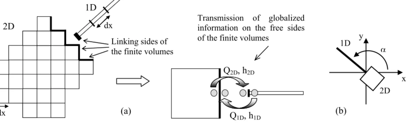
The same finite volume method is used for the spatial discretization in both the 1D and the 2D solvers. Moreover, temporal integration schemes can both be explicit. Thanks to these common features, the linking of the models is easily achieved by working at each time step on the control volumes boundaries at the domains extremities (Fig. 2 - a).

Figure 2: Principle of the model linking (a) and definition of the 1D reach angle α compared to the 2D axis (b)

Information in the cells at the 2D domain extremities are used to evaluate unknown boundary conditions for the 1D model and vice-versa. This exchange of information is performed in order to conserve the discharge as well as the momentum direction and the free surface level across linking boundaries. For the 1D model, no degree of freedom exists and the linking conditions are simply the discharge across the 2D boundary and the 2D mean free surface elevation. For the 2D model, the direction α of the flow from the 1D model, defined by the modeller, can be taken into account (Fig. 2 - b). The 2D discharge components Qx,2D and Qy,2D along x and y axis are first evaluated to keep the 1D discharge Q1D direction:

,2 1 1 1 tan x D D Q Q α = + and ,2 1 tan 1 tan y D D Q Q α α = + (6)

In a second time, they are used to compute the specific discharges qx,i and qy,i for each 2D boundary side

i by keeping a constant flow velocity and the 1D free surface elevation. The latter is used to compute the 2D

flow section Ω2D and the local height hi. , ,2 j i j D i q =V h with ,2 ,2 ,2 j D j D j D Q V = Ω and j = x ,y (7)

3. TEST

CASES

3.1 Mobile hydraulic jump

To validate the multiblock approach, the propagation of a moving hydraulic jump in a smooth and horizontal channel with a constant rectangular cross-section has been computed. In such a particular channel, considering a hydraulic jump moving with constant velocity W along the channel axis, the mass and momentum equations provides analytical data for the validation of the numerical approach.

The computation has been performed for a 50 m long channel, 3 m wide. No friction has been taken into account. The velocity of the hydraulic jump is considered as 2 m/s and the water depth is 1 m upstream and 5 m downstream. Thus, the specific discharges have to be 14.13 and 22.12 m²/s respectively upstream and downstream of the hydraulic jump for the amplitude of the shock to be constant along time. Upstream boundary conditions are the specific discharge and the water depth (supercritical flow) and the downstream

2D

1D

dx

dx

Linking sides of the finite volumes

Transmission of globalized information on the free sides of the finite volumes

Q2D, h2D Q1D, h1D α x 2D 1D y (b) (a)

h = cst

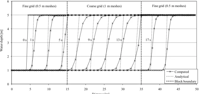
one is the water depth (subcritical flow). The initial condition corresponds to an instantaneous hydraulic jump location 4.5 m from the upstream limit of the channel. The multiblock grid covers the channel with two 15-m long reaches and a 0.5 m mesh size on either side of a central 20-m long reach with coarse meshes of 1 m. Fluxes reconstruction is constant inside a block and linear at the boundaries. Thus, the discretization scheme is first order accurate. The time integration scheme is second order accurate.

The computation has been carried out for a period of 20 s. This allows the hydraulic jump to propagate across most of the channel length and to cross twice a boundary between blocks. In the first time from the fine to the coarse grid and the second time for the coarse to the fine one. The comparison between the instantaneous free surface distributions computed analytically and with the numerical model is excellent (Fig. 3). The velocity of the moving shock and its amplitude are very well reproduced in the whole of the numerical results, even across the block boundaries. The effect of the linear reconstruction at the block boundary is visible with a local stiffening of the shock, but the instantaneous hydraulic jump profile is very similar inside the whole of the three blocks

Figure 3: Propagation of a mobile hydraulic jump in a smooth horizontal channel - Analytical and numerical results with multiblock grid

3.2 Linked models

To validate the linking approach, a winding river reach has been modelled with the 2D model and the propagation of a flood has been simulated as a reference configuration. In a second time, the upstream and downstream parts of the reach have been modelled with the 1D model and linked to a central 2D reach (Fig. 4). The simulation in this new model of the propagation of the flood provides validation of the linking procedure by comparison of the hydrodynamic parameters evolution in the central area.

Figure 4: Sketch of the simulation domain for totally 2D and coupled 1D-2D computations

Meshes 1 m in side have been used for 1D and 2D discretizations. The reach was 10 m wide and 280 m long, without bottom slope and had a rectangular cross-section. The length of the 1D reaches was 90 m. The

0 1 2 3 4 5 6 0 5 10 15 20 25 30 35 40 45 50 W at er d ept h [ m ] Distance [m] Computed Analytical Block boundary 0 s 1 s 5 s 9 s 13 s 17 s

Fine grid (0.5 m meshes) Coarse grid (1 m meshes) Fine grid (0.5 m meshes)

A B Points of validation 1D reach 2D reach Linking place Upstream Q t Downstream

initial condition was a steady flow of 10 m³/s in the reaches with a water height of 1 m downstream. Manning’s roughness coefficient was 0.04 s/m1/3 _{for the 2D domain, and 0.054 s/m}1/3 _{for the 1D one. The} latter value has been calibrated to have the same free surface level in the coupled model as in the full 2D one. The downstream boundary condition remained constant along time during all the simulations.

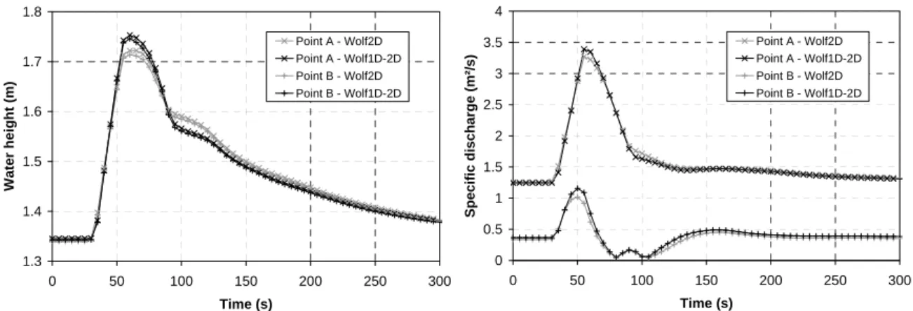
Two points (A and B, fig. 4) have been chosen for results comparison. They were respectively located in te outer and the inner parts of the central bend. The time evolution of the water height and the absolute specific discharge at these points is presented in figure 5. Time evolution of the flow variables is similar. Only a small difference in the amplitude of the peaks can be observed, but it doesn’t undermine the approach. No spurious effect of reflection or waves is generated in the linking zone. 2D hydrodynamic effects are very well reproduced, as shown by the discharge evolution to point B. Moreover, the number of calculation meshes is 2860 for the fully 2D model against 1346 for the coupled one. Thanks to this, calculation time to simulate 600 s of real time is 195.32 s in the first case and 84.67 s in the second one. The coupled approach is thus very efficient to decrease memory requirements and computation time of 2D simulations without degrading the results near interesting places.

Figure 5: Water height and specific discharge evolution at points A and B - Comparison of the two models

4. APPLICATIONS

4.1 Locks operation

The linked model has been applied to the simulation of the propagation of the waves following the filling and emptying operations of a large locks system. The goal of the study was to assess the effects in terms of water heights and velocity field of the building of a fourth 225 x 25 m lock near the existing three locks of Lanaye on the river Meuse in Belgium. Downstream of the plant, a channel links the locks to a 14 km long reach of river Meuse with a mobile dam at each extremity. A wetland is located on the right side of the river, in front of the confluence with the lock channel (Fig. 6). This complex layout leads to the propagation and the reflection of multiple waves when emptying the locks, the study of which is of great interest to assess ship navigation conditions, mobile dam operation rules as well as structures design.

Figure 6: Sketch and 2D topography of the simulation domain for the study of the area downstream of the locks 0 0.5 1 1.5 2 2.5 3 3.5 4 0 50 100 150 200 250 300 Time (s) Specif ic discharge ( m ²/ s) Point A - Wolf2D Point A - Wolf1D-2D Point B - Wolf2D Point B - Wolf1D-2D 1.3 1.4 1.5 1.6 1.7 1.8 0 50 100 150 200 250 300 Time (s) Water height (m) Point A - Wolf2D Point A - Wolf1D-2D Point B - Wolf2D Point B - Wolf1D-2D Meuse river Channel Confluence Wetland Locks 4 km 1D reach 2D domain 6 km 1D reach A B C

The field near the locks and the confluence of the channel and the river have to be modelled in 2D to correctly represent flow patterns and waves propagation. On the other hand, it is necessary to model the whole river reach to take into account waves reflection against mobile dams. Indeed, their travelling time in the domain has the same order of magnitude as the time to empty a lock. The use of the coupled 1D-2D model proved thus helpful to effectively simulate the flow field in such extended geometric pattern. An area 5 km long and 1 km wide has been modelled in 2D with +/- 60 000 square meshes from 2 x 2 m up to 16 x 16 m. It included the lock and the downstream channel, 3 km of the Meuse river reach and the wetland. The rest of the Meuse reach has been modelled in 1D with 2500 finite volumes 4 m long (Fig. 6).

Several simulations have been performed, with different scenarios for locks operation, discharge in the river Meuse… For each case, the time evolution of pertinent flow variables at strategic points has been analyzed (Fig. 7) in order to assess the effects of the new lock. 2D flow patterns have also been used to assess ship navigation conditions, especially at the confluence, and validate the hydraulic structures design.

Figure 7: Example of results: mass oscillations between the lock channel - point A - and the wetland - point B - (left) and wave reflection against downstream mobile dam (right) to point C (Fig. 6)

4.2 Flow over a smooth curved spillway

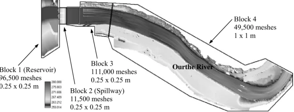
Located on the upstream part of the Ourthe River in Belgium, the 21-m high Nisramont dam is equipped with three 12.5 m wide bays on a crested weir upstream of a smooth spillway. To assess the hydraulic capacities of the system and to verify the design of the stilling basin, flows on the whole structure have been modelled in a single domain using the 2D multiblock multimodel approach. The simulation domain (Fig. 8) covered 700 m of the river, 50 m upstream and 650 m downstream of the dam crest, and was based on a very accurate and dense digital elevation model. In order to minimize CPU time while keeping good accuracy in the critical part of the domain, four different blocks with varied mesh size were defined for the computation (Fig. 9). In addition, standard SWE model was solved in blocks 1, 3 & 4 while a curvilinear coordinates based approach [1] has been applied on the spillway (block 2). Boundary conditions were deduced from large scale simulation of the whole reservoir or from data of a limnimetric station.

Figure 9: Plane view of the topography used for the simulation and blocks layout 45.95 46 46.05 46.1 46.15 46.2 46.25 0 600 1200 1800 2400 3000 3600 Temps (s) Fr ee sur face level (m ) 0 0.05 0.1 0.15 0.2 0.25 Absolute velocity (m /s)

Free surf level Velocity 45.8 45.9 46 46.1 46.2 46.3 46.4 0 600 1200 1800 2400 3000 3600 Time (s) Fr ee sur face level (m ) Locks Flooded area Initial positive wave Reflected negative wave

Out of phase free surface level variations Block 4 49,500 meshes 1 x 1 m Block 3 111,000 meshes 0.25 x 0.25 m Block 2 (Spillway) 11,500 meshes 0.25 x 0.25 m Ourthe River Block 1 (Reservoir) 96,500 meshes 0.25 x 0.25 m

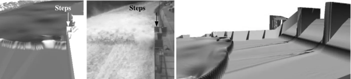
Simulation of the well documented 175 m³/s flood of the 3 January 2003 leads to very good agreement between numerical results and observations of the real event. For example, the position of the hydraulic jump at the downstream extremity of the stilling basin is reliably modeled (Fig. 10). On the basis of pictures, the real position of the flow discontinuity was approximatively 31 m downstream of the spillway toe. The numerical result is 29 m. Cross waves shape and length were compared, as well as dried areas at the bottom of the spillway piles and the reservoir water elevation. Moreover, water levels reached in the river downstream of the dam were in good agreement with those measured in reality.

Figure 10: Comparison of the hydraulic jump location in the stilling basin for a 175 m³/s flood (left) and 3D view of the numerical results on the spillway and the stilling basin (right)

5. CONCLUSIONS

The linking in the same computational domain of different flow solvers, each one used in the part of the simulation where its characteristics are most suitable, opens the door to effective flow simulations in large domains with geometrically complex boundaries. The 1D and the 2D models presented in this paper, based on mass and momentum conservation equations, use the same finite volume technique together with the same flux vector splitting and explicit time integration scheme. This makes their linking easy and ensures its physical meaning. In addition, the 2D model uses multiblock regular grids, enabling to change the mesh size in different locations of the computation area as well as the mathematical model to be solved.

The multiblock / multimodel approach and the linking procedure are shown to be efficient to simulate in a unified way very large free surface flow hydraulic systems with a very fine discretization and/or sophisticated mathematical models in local areas, without decreasing the models reliability and precision nor prohibitively increasing calculation time and memory requirements.

REFERENCES

[1] Dewals, B.J., Erpicum, S., Archambeau, P., Detrembleur, S., & Pirotton, M. (2006). Depth-integrated flow modeling taking into account bottom curvature. Journal of Hydraulic Research, 44(6), 787-795. [2] Dewals, B.J., Erpicum, S., Archambeau, P., Detrembleur, S., & Pirotton, M. (2008). Hétérogénéité des

échelles spatio-temporelles d’écoulements hydrosédimentaires et modélisation numérique. La Houille

Blanche, 5, 109-114.

[3] Dewals, B.J., Kantoush, S., Erpicum, S., Pirotton, M., & Schleiss, A. (2008). Experimental and numerical analysis of flow instabilities in rectangular shallow basins. Env. Fluid Mech., 8, 31-54.

[4] Erpicum, S., Archambeau, P., Dewals, B.J., Detrembleur, S., & Pirotton, M., (2005). Optimisation of hydroelectric power satations operations with WOLF package. Proc. of the 5th

Int. Conf. on Hydropower. Stavanger, Norway.

[5] Erpicum, S., Meile, T., Dewals, B.J., Pirotton, M., & Schleiss, A. (2009). 2D numerical flow modeling in a macro-rough channel. Int. J. for Numerical Methods in Fluids, 61(11), 1227-1246.

[6] Erpicum, S., Dewals, B.J., Archambeau, P., Detrembleur, S., & Pirotton, M. (in press). Detailed inundation modeling using high resolution DEMs. Eng. Appl. of Comp. Fluid Mech.

[7] Erpicum, S., Dewals, B.J., Archambeau, P., & Pirotton, M. (in press). Dam-break flow computation based on an efficient flux-vector splitting. Journal of Computational and Applied Mathematics.