C
hapter
2
Stratospheric Ozone and Surface
Ultraviolet Radiation
Coordinating Lead Authors:
A. Douglass V. Fioletov Lead Authors: S. Godin-Beekmann R. Müller R.S. Stolarski A. Webb Coauthors: A. Arola J.B. Burkholder J.P. Burrows M.P. Chipperfield R. Cordero C. David P.N. den Outer S.B. Diaz L.E. Flynn M. Hegglin J.R. Herman P. Huck S. Janjai I.M. Jánosi J.W. Krzyścin Y. Liu J. Logan K. Matthes R.L. McKenzie N.J. Muthama I. Petropavlovskikh M. Pitts S. Ramachandran M. Rex R.J. Salawitch B.-M. Sinnhuber J. Staehelin S. Strahan K. Tourpali J. Valverde-Canossa C. Vigouroux Contributors: G.E. Bodeker T. Canty H. De Backer P. Demoulin U. Feister S.M. Frith J.-U. Grooß F. Hase J. Klyft T. Koide M.J. Kurylo D. Loyola C.A. McLinden I.A. Megretskaia P.J. Nair M. Palm D. Papanastasiou L.R. Poole M. Schneider R. Schofield H. Slaper W. Steinbrecht S. Tegtmeier Y. Terao S. Tilmes D.I. Vyushin M. Weber E.-S. Yang
STRATOSPHERIC OZONE AND SURFACE ULTRAVIOLET RADIATION Contents SCIENTIFIC SUMMARY ...1 INTRODUCTION ...5 2.1 OzONE OBSERVATIONS ...5 2.1.1 State of Science in 2006 ...5
2.1.2 Update on Methods Used to Evaluate the Effect of ODSs on Ozone ...5
2.1.3 Update on Total Ozone Changes ...6
2.1.3.1 Measurements ...6
2.1.3.2 Total Ozone Changes and Trends ...8
2.1.4 Update on Ozone Profile Changes ...10
2.1.4.1 Measurements ...10
2.1.4.2 Ozone Profile Changes ...12
2.2 POLAR OzONE ...17
2.2.1 State of Science in 2006 ...17
2.2.2 Polar Ozone Chemistry ...18
2.2.2.1 Laboratory Studies of the ClOOCl UV Absorption Spectrum ...19
2.2.2.2 Field Observations of Chlorine Partitioning ...21
2.2.2.3 Other Issues Related to Polar Ozone Chemistry ...25
2.2.3 Polar Stratospheric Cloud Processes ...25
2.2.3.1 New Observational Data Sets ...26
2.2.3.2 PSC Composition ...27
2.2.3.3 PSC Forcing Mechanisms ...27
2.2.3.4 Use of Proxies to Represent PSC Processes ...28
2.2.4 Arctic Polar Temperatures and Ozone ...29
2.2.5 Antarctic Polar Temperatures and Ozone ...30
2.2.6 The Onset of Antarctic Ozone Depletion ...31
2.3 SURFACE ULTRAVIOLET RADIATION ...31
2.3.1 State of Science in 2006 ...31
Box 2-1Radiation Amplification Factor for Erythemal Irradiance ...32
2.3.2 Update on Factors Affecting UV Radiation ...33
2.3.2.1 Ozone Effects ...33
2.3.2.2 Other Influences on UV ...34
2.3.3 Ground-Based and Satellite UV Data ...35
2.3.3.1 Ground-Based UV Measurements ...35
2.3.3.2 Ground-Based UV Reconstruction ...35
2.3.3.3 UV Estimates from Satellite Observations ...36
2.3.4 Long-Term Changes in UV ...37
2.3.4.1 Ground-Based Observations ...37
2.3.4.2 Reconstructed UV Data ...38
2.3.4.3 Satellite Estimates of Irradiance Changes ...40
2.3.4.4 Consistency of UV Estimates from Observations, Reconstructions, and Satellite Data ...41
2.4 INTERPRETATION OF OBSERVED OzONE CHANGES ...41
2.4.2.1 Update from JPL 2002 to JPL 2006 ...43
2.4.2.2 Updates since JPL 2006 ...43
2.4.3 The Distribution and Variability of Stratospheric Ozone and Their Representation in Models ...44
2.4.3.1 Annual Cycle and Natural Variability ...44
2.4.3.2 Solar Cycle ...44
2.4.3.3 Volcanic and Aerosol Effects ...46
2.4.3.4 Evaluation of Simulated Transport ...47
2.4.3.5 Evaluation of the Chemical Mechanism and Its Implementation ...49
2.4.3.6 Evaluation of Simulations of the Upper Troposphere/Lower Stratosphere ...49
2.4.4 Recovery Detection and Attribution...50
2.4.4.1 Dynamical Contributions to Apparent Trend ...50
2.4.4.2 Greenhouse Gas Effects on Ozone Trends ...50
2.4.4.3 Polar Loss and Dilution to Midlatitudes ...51
2.4.5 Simulation of Ozone Changes for the Last Three Decades...51
2.4.5.1 Total Ozone Trends ...51
2.4.5.2 Midlatitude Profile Trends ...53
2.4.5.3 Tropical Profile Trends ...55
2.4.5.4 Polar Trends ...55
2.4.5.5 Trends and Recovery in the Upper Troposphere and Lower Stratosphere ...58
SCIENTIFIC SUmmARy
Global Ozone Observations and Interpretation
As a result of the Montreal Protocol, ozone is expected to recover from the effect of ozone-depleting substances (ODSs) as their abundances decline in the coming decades. The 2006 Assessment showed that globally averaged column ozone ceased to decline around 1996, meeting the criterion for the first stage of recovery. Ozone is expected to increase as a result of continued decrease in ODSs (second stage of recovery). This chapter discusses recent observations of ozone and ultraviolet radiation in the context of their historical records. Natural variability, observational uncertainty, and stratospheric cooling necessitate a long record in order to attribute an ozone increase to decreases in ODSs. Table S2-1 summarizes ozone changes since 1980.
The primary tools used in this Assessment for prediction of ozone are chemistry-climate models (CCMs). These CCMs are designed to represent the processes determining the amount of stratospheric ozone and its response to changes in ODSs and greenhouse gases. Eighteen CCMs have been recently evaluated using a variety of process-based compari-sons to measurements. The CCMs are further evaluated here by comparison of trends calculated from measurements with trends calculated from simulations designed to reproduce ozone behavior during an observing period.
Total Column Ozone
• Average total ozone values in 2006–2009 have remained at the same level for the past decade, about 3.5% and 2.5% below the 1964–1980 averages respectively for 90°S–90°N and 60°S–60°N. Average total ozone from
CCM simulations behaves in a manner similar to observations between 1980 and 2009. The average column ozone for 1964–1980 is chosen as a reference for observed changes for two reasons: 1) reliable ground-based observa-tions sufficient to produce a global average are available in this period; 2) a significant trend is not discernible in the observations during this period.
• Southern Hemisphere midlatitude (35°S–60°S) annual mean total column ozone amounts over the period 2006–2009 have remained at the same level as observed during 1996–2005, approximately 6% below the 1964–1980 average. Simulations by CCMs also show declines of the same magnitude between 1980 and 1996, and
minimal change after 1996, thus both observations and simulations are consistent with the expectations of the impact of ODSs on southern midlatitude ozone.
• Northern Hemisphere midlatitude (35°N–60°N) annual mean total column ozone amounts over the period 2006–2009 have remained at the same level as observed during 1998–2005, approximately 3.5% below the 1964–1980 average. A minimum about 5.5% below the 1964–1980 average was reached in the mid-1990s.
Simulations by CCMs agree with these measurements, again showing the consistency of data with the expected impact of ODSs. The simulations also indicate that the minimum in the mid-1990s was primarily caused by the ozone response to effects of volcanic aerosols from the 1991 eruption of Mt. Pinatubo.
• The latitude dependence of simulated total column ozone trends generally agrees with that derived from measurements, showing large negative trends at Southern Hemisphere mid and high latitudes and Northern Hemisphere midlatitudes for the period of ODS increase. However, in the tropics the statistically significant
range of trends produced by CCMs (−1.5 to −4 Dobson units per decade (DU/decade)) does not agree with the trend obtained from measurements (+0.3 ± 1 DU/decade).
Ozone Profiles
• Northern Hemisphere midlatitude (35°N–60°N) ozone between 12 and 15 km decreased between 1979 and 1995, and increased between 1996 and 2009. The increase since the mid-1990s is larger than the changes expected
• Northern Hemisphere midlatitude (35°N–60°N) ozone between 20 and 25 km declined during 1979–1995 and has since ceased to decline. Observed increases between 1996 and 2008 are statistically significant at some locations but
not globally.
• Northern Hemisphere midlatitude (35°N–60°N) ozone between 35 and 45 km measured using a broad range of ground-based and satellite instruments ceased to decline after the mid-1990s, consistent with the leveling off of ODS abundances. All data sets show a small ozone increase since that time, with varying degrees of statistical
significance but this increase cannot presently be attributed to ODS decrease because of observational uncertainty, natural ozone variability, and stratospheric cooling. CCMs simulate the ozone response to changes in ODSs and increases in greenhouse gases; analysis of CCM results suggests that longer observational records are required to separate these effects from each other and from natural variability.
• In the midlatitude upper stratosphere (35–45 km) of both hemispheres, the profile ozone trends derived from most CCMs from 1980 to 1996 agree well with trends deduced from measurements. The agreement in both
mag-nitude and shape of the ozone trends provides evidence that increases in ODSs between 1980 and 1996 are primarily responsible for the observed behavior.
• In the tropical lower stratosphere, all simulations show a negative ozone trend just above the tropopause, centered at about 18–19 km (70–80 hectoPascals, hPa), due to an increase in upwelling. The simulated trends in
the lower tropical stratosphere are consistent with trends deduced for 1985–2005 from Stratospheric Aerosol and Gas Experiment (SAGE II) satellite data, although uncertainties in the SAGE II trends are large. The near-zero trend in tropical total ozone measurements is inconsistent with the negative trend found in the integrated SAGE I + SAGE II stratospheric profiles. The tropospheric ozone column does not increase enough to resolve this discrepancy.
Table S2-1. Summary of ozone changes estimated from observations.
Column Ozone 12–15 km 20–25 km 35–45 km Comment
Data Sources Ground-based, satellite Ozonesondes Ozonesondes,satellites, FTIR Satellites, Umkehrs, FTIR Northern midlatitudes 1980–1996 Declined by
about 6% Declined by about 9% Declined by about 7% Declined by about 10%
1992–1996 column and lower stratosphere data affected by Mt. Pinatubo Northern midlatitudes 1996–2009 Increased from the minimum values by about 2% by 1998 and remained at the same level thereafter
Increased by
about 6% Increased byabout 2.5%
Increased by 1 to 2%, but uncertainties are large Southern midlatitudes
1980–1996 Declined by 6% No information Declined by about 7%
Declined by about 10% Southern midlatitudes 1996–2009 Remained at approximately the same level
No statistically significant changes No statistically significant changes Increased by 1 to 3%, but uncertainties are large
Polar Ozone Observations and Interpretation
• The Antarctic ozone hole continued to appear each spring from 2006 to 2009. This is expected because decreases
in stratospheric chlorine and bromine have been moderate over the last few years. Analysis shows that since 1979 the abundance of total column ozone in the Antarctic ozone hole has evolved in a manner consistent with the time evolution of ODSs. Since about 1997 the ODS amounts have been nearly constant and the depth and magnitude of the ozone hole have been controlled by variations in temperature and dynamics. The October mean column ozone within the vortex has been about 40% below 1980 values for the past fifteen years.
• Arctic winter and spring ozone loss has varied between 2007 and 2010, but remained in a range comparable to the values that have prevailed since the early 1990s. Chemical loss of about 80% of the losses observed in the
record cold winters of 1999/2000 and 2004/2005 has occurred in recent cold winters.
• Recent laboratory measurements of the chlorine monoxide dimer (ClOOCl) dissociation cross section and analyses of observations from aircraft and satellites have reaffirmed the fundamental understanding that polar springtime ozone depletion is caused primarily by the ClO + ClO catalytic ozone destruction cycle, with significant contributions from the BrO + ClO cycle.
• Polar stratospheric clouds (PSCs) over Antarctica occur more frequently in early June and less frequently in September than expected based on the previous satellite PSC climatology. This result is obtained from
measure-ments by a new class of satellite instrumeasure-ments that provide daily vortex-wide information concerning PSC composition and occurrence in both hemispheres. The previous satellite PSC climatology was developed from solar occultation instruments that have limited daily coverage.
• Calculations constrained to match observed temperatures and halogen levels produce Antarctic ozone losses that are close to those derived from data. Without constraints, CCMs simulate many aspects of the Antarctic
ozone hole, however they do not simultaneously produce the cold temperatures, isolation from middle latitudes, deep descent, and high amounts of halogens in the polar vortex. Furthermore, most CCMs underestimate the Arctic ozone loss that is derived from observations, primarily because the simulated northern winter vortices are too warm.
Ultraviolet Radiation
Ground-based measurements of solar ultraviolet (UV) radiation (wavelength 280–400 nanometers) remain limited both spatially and in duration. However, there have been advances both in reconstructing longer-term UV records from other types of ground-based measurements and in satellite UV retrievals. Where these UV data sets coincide, long-term changes agree, even though there may be differences in instantaneous, absolute levels of UV.
• Ground-based UV reconstructions and satellite UV retrievals, supported in the later years by direct ground-based UV measurements, show that erythemal (“sunburning”) irradiance over midlatitudes has increased since the late 1970s, in qualitative agreement with the observed decrease in column ozone. The increase in
satellite-derived erythemal irradiance over midlatitudes during 1979–2008 is statistically significant, while there are no significant changes in the tropics. Satellite estimates of UV are difficult to interpret over the polar regions.
• In the Antarctic, large ozone losses produce a clear increase in surface UV radiation. Ground-based
measure-ments show that the average spring erythemal irradiance for 1990–2006 is up to 85% greater than the modeled irradiance for 1963–1980, depending on site. The Antarctic spring erythemal irradiance is approximately twice that measured in the Arctic for the same season.
• Clear-sky UV observations from unpolluted sites in midlatitudes show that since the late 1990s, UV irradiance levels have been approximately constant, consistent with ozone column observations over this period.
• Surface UV levels and trends have also been significantly influenced by clouds and aerosols, in addition to stratospheric ozone. Daily measurements under all atmospheric conditions at sites in Europe and Japan show that
erythemal irradiance has continued to increase in recent years due to net reductions in the effects of clouds and aero-sols. In contrast, in southern midlatitudes, zonal and annual average erythemal irradiance increases due to ozone decreases since 1979 have been offset by almost a half due to net increases in the effects of clouds and aerosols.
INTRODUCTION
This chapter presents information on several topics but is conceptually organized around a single question: is the Montreal Protocol working? This chapter is focused on the observational record and interpretation thereof up to the present, and consolidates information found in three separate chapters in the previous Assessment (WMO, 2007): Chapter 3 (“Global Ozone: Past and Present,” Chipperfield and Fioletov et al., 2007), Chapter 4 (“Polar Ozone: Past and Present,” Newman and Rex et al., 2007) and Chapter 7 (“Surface Ultraviolet Radiation: Past, Pres-ent and Future,” Bais and Lubin et al., 2007). There are four sections in this chapter: Ozone Observations, Polar Ozone, Surface Ultraviolet Radiation, and Interpretation of Observed Ozone Changes. Each section begins with a summary of WMO (2007) followed by a combination of updates to the observational records and longer discussion of new discoveries and observations.
2.1 OZONE ObSERVATIONS 2.1.1 State of Science in 2006
The long-term changes in global ozone were re-viewed in Chapter 3 of WMO (2007). From the analysis of data from multiple sources, it was shown that the global mean total column ozone values for the period 2002–2005 had stabilized to values similar to those observed in 1998– 2001, at approximately 3.5% below the 1964–1980 average values. Differences between the Northern and Southern Hemispheres (NH and SH) were noted, with ozone aver-age values respectively 3% and 5.5% below their pre-1980 average values. The time series behavior of total ozone column was also shown to be different in both hemispheres during the 1990s. Ozone showed a minimum in the NH around 1993 followed by an increase, while it decreased through the late 1990s in the SH and leveled off in about 2000. Seasonal differences between ozone changes over midlatitude regions in both hemispheres were also noticed. The changes with respect to the pre-1980 values were larg-er in spring in the NH, while no seasonal dependence was found in the SH. Over the tropics, no change in column ozone values was found, which was consistent with the findings of WMO (2003).
Because total ozone column was no longer decreas-ing in most observations, several methods were discussed in WMO (2003) and WMO (2007) for the evaluation of ozone trends. Previous Assessments had described long-term ozone changes due to chemical destruction by ozone-depleting substances (ODSs) in terms of linear trends estimated using multiple regression analysis. Because the change in ODSs after the mid-1990s was no longer linear
with time, other methods were proposed, e.g., the piece-wise linear trend model in which different linear fits are used before and after a turning point, and the fit to the equivalent effective stratospheric chlorine (EESC) func-tion (see Chapter 1 of this Assessment). Such methods have been used in most recent studies on ozone trends and are also discussed in the present Assessment.
Regarding changes in the vertical ozone distribu-tion, satellite and ground-based measurements showed that in the upper stratosphere, the ozone decrease had stopped and ozone values were relatively constant since 1995. Similar stabilization was found in the lower strato-sphere between 20 and 25 kilometers (km) altitude. In the lowermost stratosphere below 15 km altitude in the NH, a significant increase was found from 1996, after the strong decrease observed between 1979 and 1995. This change in the lowermost stratosphere had a substantial impact on the total ozone column. Such an ozone increase was not observed in the SH. The lowermost stratosphere is de-fined and discussed in more detail in Section 2.4 below.
All studies in WMO (2007) pointed out the stabi-lization of ozone both in total column and in the vertical distribution at various levels, various locations, and at the global scale. They concurred that the first stage of recov-ery (i.e., slowing of ozone decline attributable to ODS changes) had already occurred and that the second stage (i.e., onset of ozone increase) was expected to become evi-dent within the next two decades.
2.1.2 Update on methods Used to Evaluate the Effect of ODSs on Ozone
As discussed in previous Assessments, the long-term and short-long-term variability of ozone in the strato-sphere is generally estimated using multi-regression statis-tical models that quantify the relationship between ozone and different explanatory variables describing natural or anthropogenic forcings (e.g., SPARC, 1998). The long-term trend components representing the effect of ODSs are extracted simultaneously with other regression terms and autocorrelated noise.
To describe the long-term trend in ozone that is related to ODSs, the equivalent effective stratospheric chlorine (EESC) (see Section 1.4.4 of Chapter 1) is com-monly used as a proxy in statistical models (Stolarski et al., 2006; Dhomse et al., 2006; Brunner et al., 2006; Randel and Wu, 2007; Wohltmann et al., 2007; Mäder et al., 2007; Vyushin et al., 2007; Harris et al., 2008). Statistical methods are used to quantify the relationship between ozone changes and EESC, and verify whether the EESC-related term is statistically significant. Analysis of the residuals, for example, by the Cumulative Sum of Residuals (CUSUM) technique (Reinsel et al., 2002;
Newchurch et al., 2003) then can be used to check that a statistical model with the EESC term adequately describes the observed ozone changes.
The EESC depends on latitude and altitude. More-over, the present estimates of EESC are different from those used, for example, in WMO (2003) as discussed in Section 1.4.4 of Chapter 1. As a result, all of the ozone trend studies mentioned above did not use the same EESC function. While a particular shape of the EESC curve has little effect on the EESC-based trend estimates in the past (they all represent a linear decline during the 1980s and early 1990s with leveling off thereafter), the shape of an EESC function will have more impact on the estimated trend value as time moves from the EESC turning point. The shape of the EESC curve is particularly important for the detectability of future trends (Vyushin et al., 2010). On the other hand, once the EESC shape is specified, the sensitivity of ozone to EESC obtained from this type of statistical analysis varies little as a result of small differ-ences in the length of record.
A statistically significant EESC-related term can be used as evidence of the ODS-related destruction of ozone. The EESC was a linear function of time in the 1980s and thus the EESC fit to ozone can be expressed in terms of linear changes at that time, with results reported in ozone changes (% or Dobson units (DU)) per decade. WMO (2007, Section 3.2.1) discussed ozone trends in terms of EESC. Adding four more years to 25-year-long observa-tion records discussed in WMO (2007) does not change the trend estimates for that period significantly. Simi-larly, the EESC is nearly a linear function in the 2000s and therefore the expected rate of ozone increase during the declining phase of the EESC can be expressed in % or DU per decade.
WMO (2007) concluded that the first stage of the ozone recovery, i.e., the slowing of ozone decline, identi-fied as the occurrence of a statistically significant reduc-tion in the rate of decline in ozone due to changing EESC, had already occurred. The second stage of the ozone re-covery or the onset of ozone increases (turnaround) is identified as the occurrence of statistically significant increases in ozone above previous minimum values due to declining EESC.
The ozone increase after the minimum can be estimated by fitting the data with a linear function or by calculating a piecewise linear trend (PWLT) with a turn-ing point near the EESC maximum (Reinsel et al., 2005; Miller et al., 2006; Vyushin et al., 2007; S.-K. Yang et al., 2009). The slope estimated from ozone data during the declining phase of EESC should agree with the slope expected from the EESC fit if the ozone increase is indeed related to the EESC decline.
As discussed by WMO (2007, Section 3.4.2) a siz-able fraction of the long-term ozone changes, particularly
over northern mid and high latitudes, can be related to dynamical processes. Estimation of ozone trends requires a proper accounting for the effect of these processes on ozone. One approach is to add more terms to the sta-tistical model used for trend calculations using a purely statistical approach and letting the regression model find the best proxies (e.g., Mäder et al., 2007) or by adding proxies based on possible physical processes that cause the ozone changes (e.g., Wohltmann et al., 2007). How-ever the physical mechanisms underlying these additional terms are often not well understood, and therefore it is dif-ficult to account for them properly in a statistical model. This issue is addressed in detail in Section 2.4. Another approach is to consider the contribution from dynamical processes as noise. This results in a larger uncertainty in the trend estimates and also requires an additional analysis of the autocorrelation function of the residuals (Vyushin et al., 2007). In both approaches, the eleven-year solar activity cycle and the quasi-biennial oscillation (QBO) are typically included in the statistical model because these oscillations are located in a narrow frequency range.
2.1.3 Update on Total Ozone Changes 2.1.3.1 MeasureMents
Ground-Based Measurements
Dobson, Brewer, and filter instruments provide long-term ground-based total ozone time series. The instrumental precision of well maintained Dobson and Brewer instruments was recently estimated by Scarnato et al. (2010) to be respectively 0.5% and 0.15% (1-sigma). When comparing ground-based total ozone measurements with satellite overpass data, the standard deviation of monthly differences was on average about 1.5% and within 0.6–2.6% for 90% of Dobson and Brewer network stations and on average about 2% and within 1.5–3.5% for 90% of stations equipped with filter instruments M-124 (Fioletov et al., 2008). The agreement between various instruments can be further improved as new ozone absorption cross sections are adopted (Scarnato et al., 2009). A recently established committee is presently addressing the issue of ozone cross sections used in ground-based and satellite measurements (see http://igaco-o3.fmi.fi/ACSO/). Since the end of the 1980s, other instruments have been imple-mented for the monitoring of total ozone. Long-term and regular ground-based Fourier transform infrared (FTIR) measurements are performed at many stations around the world and these data were used to assess ozone trends over Western Europe from 79°N to 28°N (Vigouroux et al., 2008). The precision of FTIR ozone total columns
is about 4%, but it has been demonstrated that it can reach 1 DU in some conditions (Schneider et al., 2008). No calibration is needed, but the instrumental line shape must be known in order to avoid introducing a bias in the ozone retrievals. UV-Visible spectrophotometers such as the System d’ Analyse par Observation zenitale (SAOz) instruments (Pommereau and Goutail, 1988) retrieve total ozone as well as nitrogen dioxide (NO2) column amounts
from zenith sky measurements using the Differential Opti-cal Absorption Spectroscopy (DOAS). A new version of the zenith-sky retrieval algorithm using improved air mass factors was recently introduced. SAOz observations were used here in addition to Dobson, Brewer, and filter instru-ment data to form the ground-based zonal mean data set as described by Fioletov et al. (2002). This data set with the list of contributed stations is available from http://woudc. org/data_e.html.
Satellite Measurements
Satellite instruments have observed the total ozone distributions at the global scale since 1970, when the Nimbus 4 satellite was launched with the Backscatter Ultraviolet (BUV) instrument onboard. To date, the long-est total ozone records are provided by the series of Total Ozone Mapping Spectrometer (TOMS) and Solar Back-scatter Ultraviolet 2 (SBUV/2) instruments. Since 2004, the TOMS total ozone record has been taken over by the Ozone Monitoring Instrument (OMI), an instrument on the Aura satellite. TOMS, BUV, and SBUV/2 data pre-sented here are retrieved with the version 8 algorithm (Bhartia et al., 2004; Flynn, 2007). There are two opera-tionally available OMI satellite total ozone column data products, based on the OMI-TOMS and the OMI-DOAS retrieval algorithms, but outputs of the OMI-TOMS algo-rithm agree better with the most accurate ground-based measurements than those for the OMI-DOAS algorithm (Balis et al., 2007). The TOMS algorithm uses only two wavelengths (317.5 and 331.2 nanometers (nm)) to derive total ozone (four other wavelengths are used for diagnos-tics and error correction). The version 8.5 OMI algorithm is similar to the TOMS version 8 algorithm and is used to process OMI data presented here.
In order to obtain long-term total ozone records, several data sets merging various satellite ozone records have been constructed. The TOMS+OMI+SBUV(/2) merged ozone data set (MOD) (Stolarski and Frith, 2006), used in WMO (2007), has been updated through Decem-ber of 2009. The input now includes version 8.5 data from OMI and version 8.0 data from NOAA 17 SBUV/2. Data from 1970 through 1972 have also been added from the Nimbus 4 BUV experiment in 1970–1977. The merged
ozone data set (MOD) can be obtained at http://acdb-ext. gsfc.nasa.gov/Data_services/merged/.
Version 8 ozone retrievals from Nimbus 7 SBUV, and NOAA-9, -11, -14, -16, -17, and -18 SBUV/2 instru-ments were used in a NOAA cohesive SBUV(/2) total ozone data set (S.K. Yang et al., 2009) available at ftp:// ftp.cpc.ncep.noaa.gov/long/SBUV_v8_Cohesive.
The European instruments Global Ozone Monitoring Experiment (GOME) on the European Remote Sensing Sat-ellite (ERS-2) (1995–2003, global coverage), Scanning Im-aging Absorption Spectrometer for Atmospheric Cartogra-phy (SCIAMACHY) on the Environmental Satellite (Envisat; 2002–present), and GOME2 on Meteorological Operational satellite (MetOp)-A (2006–present) apply the DOAS algorithm technique in the continuous 325–335 nm wavelength range (Burrows et al., 1999) to retrieve total ozone estimates. Different types of DOAS algorithms have been developed: WFDOAS (Coldewey-Egbers et al., 2005), TOGOMI/TOSOMI (Eskes et al., 2005), and SDOAS/ GDOAS/GDP (Van Roozendael et al., 2006). By compar-ing to Brewer/Dobsons and other satellite data, all algo-rithms applied to GOME were shown to be in good agree-ment (Weber et al., 2005; Balis et al., 2007; Fioletov et al., 2008). Overall good agreement was also found in the com-parison of SCIAMACHY total ozone to ground data and other satellite data over more than six years (Lerot et al., 2009). However, a downward drift of total ozone from SCIAMACHY with respect to GOME and other correlative data has been identified that is independent of the algorithm used (Lerot et al., 2009; Loyola et al., 2009a). GOME2 has almost three years of total ozone data. First validation results have been reported (Antón et al., 2009). A merged data set from GOME, SCIAMACHY, and GOME2 by suc-cessive scaling of SCIAMACHY and GOME2 monthly-mean zonal monthly-mean data to GOME is described in Loyola et al. (2009a). They report that a scaling of +2 to +3% was required to match GOME2 to the GOME data record.
The GOME-SCIAMACHY data is based on com-bined GOME, SCIAMACHY, and GOME-2 records, with SCIAMACHY and GOME-2 records adjusted using a stable record of the GOME instrument (although with a limited coverage after 2003). While multiple versions of the data processing algorithm and merged data sets exist ( Weber et al., 2007; Loyola et al., 2009a), they produce nearly identical records of zonal monthly-mean ozone values.
Measurements from four TOMS instruments, GOME, four SBUV(/2) instruments, and OMI are used to produce the New zealand National Institute of Water and Atmospheric Research (NIWA) combined total ozone data set (Bodeker et al., 2005; Müller et al., 2008). Offsets and drifts between all of the satellite-based data sets are removed through intercomparisons with the
Dobson and Brewer ground-based network. The NIWA data set is available from http://www.bodekerscientific. com/data/ozone.
2.1.3.2 total ozone Changesand trends
The quasi-global (60°S–60°N) ozone record from the MOD is shown in Figure 2-1. The annual variation and an 11-year periodical component are evident from the plot and are discussed in detail in WMO, 2007 (Chipper-field and Fioletov et al., 2007). The total ozone deviations for the 60°S–60°N, 90°S–90°N, 25°S–25°N, 35°N–60°N, and 35°S–60°S latitude belts are shown in Figure 2-2. The approach used in Fioletov et al. (2002) and WMO (2007) is again used here. Five data sets of 5°-wide zonal av-erages of total ozone values are analyzed in this Assess-ment. Area-weighted annual averages are calculated for different latitude belts and for the globe. All panels of Figure 2-2 indicate that average total ozone deviations in 2006–2009 display very little change as compared to the 2002–2005 values reported in WMO (2007). The global and 60°S–60°N averages were about 3.5% and 2.5% be-low the 1964–1980 average values, respectively. The total column ozone for 1964–1980 is chosen as a reference for observed changes for two reasons: (1) reliable ground-based observations sufficient to produce a global average are available in this period; and (2) a significant trend is not discernible in the observations during this period. In midlatitude regions of both hemispheres, ozone values in the NH and SH stabilized at respectively about 3.5% and 6% lower than the 1964–1980 average, with little sign of increase in recent years.
Several authors have examined the zonally aver-aged total ozone data and find statistically significant pos-itive trends since the second half of the 1990s. S.-K. Yang et al. (2009) find a positive trend of about 1.2 ± 0.8%/ decade for the period 1996–2007 in the averaged 50°S–50°N SBUV(/2) satellite data using the PWLT model. Using Dobson total ozone measurements, Angell and Free (2009) find positive trends in the same regions after application of 5-year running linear trends to the smoothed individual station ground-based data. They used 11-year running means to minimize the 11-year solar and QBO effects in the ozone time series. It should be mentioned however, that the positive trend in 50°S–50°N region is largely as-sociated with an ozone increase in the tropical belt related to relatively low ozone values there in the mid-1990s and relatively high values during the recent solar activity min-imum. Loyola et al. (2009b) analyzed the merged GOME(/2)+SCIAMACHY data set as well the MOD set for the period from June 1995 to April 2009. They report a statistically significant positive linear trend between 5°S and 30°N for both satellite data sets. All these findings seem to contradict previous estimates of the number of
years required to detect statistically significant ozone trend expected from the decline of ODSs (Weatherhead et al., 2000; Vyushin et al., 2007). These studies predicted that statistically significant ozone trends will be detect-able first at southern midlatitudes but that this will not be possible earlier than 2015–2020.
Comparison of the PWLT (or linear trend) esti-mates with results based on the EESC fit, shows that these recent positive ozone trends are larger than those expected from the decline in ODSs. As mentioned above, knowing the EESC decreasing rate after the turning point in the late 1990s, the corresponding linear term in total ozone regres-sion can be compared to positive trends in PWLT models. Figure 2-3 (updated Figures 8 and 9 of Vyushin et al., 2007) illustrates the ozone zonal trends by PWLT and EESC models with the solar and QBO terms applied to the MOD set for the periods 1979–2008, with the turning point for the PWLT in 1996. Figure 2-3 shows the rate of ozone increase based on the EESC fit for the period cor-responding to the declining phase of EESC and the esti-mates for the linear trend after the turning point of the PWLT. The gray areas indicate 95% confidence intervals for the PWLT estimate. The two trends are fairly similar in southern middle and high latitudes, although the uncer-tainties on the observed trends encompass zero. In north-ern middle and high latitudes, however, the observed linear trend is roughly four times the EESC-predicted trend and is actually statistically significant over northern middle and low latitudes according to the PWLT estimate of the noise. In these regions, the ODS decrease induces a positive trend but it is overwhelmed by large dynamically driven variations. This result is confirmed by several
60oS-60oN Area-Weighted Average 1970 1980 1990 2000 2010 Year 270 280 290 300 310
Total Ozone (DU)
Figure 2-1. Quasi-global (60°N–60°S) average of
to-tal ozone distribution (Dobson units) for the period 1970–2009 from the BUV/TOMS/SBUV(/2) merged ozone data set.
Stratospheric Ozone and Surface UV
authors, who indicate that the EESC decrease since the mid-1990s is not a major contributor to the recent in-crease in ozone (Reinsel et al., 2005; Dhomse et al., 2006; Wohltmann et al., 2007; and Harris et al., 2008).
On a regional scale, Krzyścin and Borkowski (2008) evaluate the ozone trend variability over Europe using 10-year blocks of reconstructed total ozone time
series since 1950. Statistically significant negative trends of 1 to 5%/decade are found almost over the whole of Europe only in the period 1985–1994. Trends up to −3%/ decade appeared over small areas in earlier periods when the anthropogenic forcing on the ozone layer was weak. Vigouroux et al. (2008) provide total ozone trends from homogenized FTIR measurements in European stations,
Ground-based dataset
NASA TOMS/OMI/SBUV merged dataset GOME/SCIAMACHY merged dataset NOAA SBUV merged dataset
NIWA Assimilated dataset
Figure 2-2. Annual mean area-weighted total ozone deviations from the 1964–1980 means for the latitude
bands 90°S–90°N, 60°S–60°N, 25°S–25°N, 35°N–60°N, and 35°S–60°S, estimated from different global da-tasets: ground-based (black), NASA TOMS/OMI/SBUV(/2) merged satellite data set (red), National Institute of Water and Atmospheric Research (NIWA) assimilated data set (magenta), NOAA SBUV(/2) (blue), and GOME/ SCHIAMACHY merged total ozone data (green). Each data set was deseasonalized with respect to the period 1979–1987. The average of the monthly-mean anomalies for 1964–1980 estimated from ground-based data was then subtracted from each anomaly time series. Deviations are expressed as percentages of the ground-based time average for the period 1964–1980. Figure updated from Chapter 3 of WMO, 2007.
over the 1995–2004 period. These trends have been up-dated for the 1995–2009 period for the present Assess-ment and are summarized in Table 2-1. Because the time series are too short to employ the multi-regression models described in Sect. 2.1.2, a bootstrap resampling method was used, which allows for non-normally distributed data and gives an independent evaluation of the uncertainty in the trend value (Gardiner et al., 2008). The total column trends are close to zero and not significant at all stations except at Kiruna, where the trend is significantly positive.
2.1.4 Update on Ozone Profile Changes 2.1.4.1 MeasureMents
Ground-Based Measurements
Ozonesondes, Dobson and Brewer spectrometers using the Umkehr method, lidars, and microwave instru-ments provide long-term measureinstru-ments of ozone vertical distribution. Various recent studies have focused on
assessing the quality and stability of ozonesonde data. Dif-ferences ranging from 5 to 10% were found between data obtained with sondes produced from different manufactur-ers or with different sensing solutions (Thompson et al., 2007; Smit et al., 2007; Kivi et al., 2007; Deshler et al., 2008; Stübi et al., 2008). The Umkehr method retrieves ozone profiles from Dobson and Brewer measurements with a vertical resolution of about 5 km in the stratosphere. Current Umkehr data are retrieved using the UMK04 algo-rithm already released for the previous Assessment ( Petropavlovskikh et al., 2005a, 2005b). Lidars and micro-wave spectrometers provide range-resolved measurements from the lower stratosphere to about 50 km for the lidar and higher for the microwave. Lidar measurements are charac-terized by a higher vertical resolution than microwave measurements, but they require clear skies so fewer mea-surements are obtained. A detailed description of the char-acteristics of ozonesondes, Umkehr, lidar, and microwave measurements in terms of accuracy and vertical resolution can be found in WMO (2007) and SPARC (1998).
A new ozone profile data source has been intro-duced for this Assessment, based on the inversion of FTIR measurements (Hase, 2000; Pougatchev et al., 1995). The
Latitude
60S 30S Eq. 30N 60N
T
otal Oz
one Anomaly (DU)
40−45S 1980 1985 1990 1995 2000 2005 2010 −5 0− 30 −1 01 0 −4 0− 20 0 40−45N 1980 1985 1990 1995 2000 2005 2010 60S 30S Eq. 30N 60N Tr end (DU/year ) Tr end (DU/year ) -0.5 0 0.5 1 1.5 2 2. 5 PWLT PWLT EESC EESC 1996-2008 1979-1995 -2 -1.5 -1 -0.5
0 Figure 2-3. (top) The EESC-based
linear trend in ozone (Dobson units/ year) calculated for the increasing part of EESC (yellow solid circles connected by the yellow line) is com-pared to the first (declining) slope of the PWLT fit for the period 1979–1995 (blue diamonds connected by the solid blue line) with 95% confidence inter-vals (gray shading) for the PWLT fit. (middle) The EESC-based linear trend in ozone (DU/year) calculated for the declining part of EESC (yellow solid circles connected by the yellow line) is compared to the second (increas-ing) slope of the PWLT fit for the pe-riod 1996–2008 (blue diamonds con-nected by the solid blue line) with 95% confidence intervals (gray shading) for the PWLT fit. (bottom) Monthly and zonal mean total ozone anomalies for the 40°S–45°S and 40°N–45°N latitude bands obtained by filtering out the seasonal cycle, QBO, and solar flux, together with the EESC (yellow) and PWLT (blue) fits. Updated from Vyushin et al. (2007). The MOD set was used.
inversion is based on the optimal estimation method (Rod-gers, 2000) and leads to 4–5 degrees of freedom in the whole column (Barret et al., 2002). Therefore, in addi-tion to total column ozone, FTIR measurements can pro-vide ozone profile data in 4 vertical layers (approximately ground–10 km; 10–18 km; 18–27 km; and 27–42 km). The precision of these four ozone partial columns is about 9.5%, 6.5%, 8.5%, and 6.0%, respectively (Vigouroux et al., 2008).
Satellite Measurements and Merged Data Sets
The second Stratospheric Aerosol and Gas Ex-periment (SAGE II) and Halogen Occultation ExEx-periment (HALOE) satellite instruments that provided long and sta-ble global observations of the ozone vertical distribution using the solar occultation technique ceased operation in 2005. Their long observational records, which were used in the previous Assessments, cover the periods 1984–2005 and 1991–2005 respectively. The longest ozone profile record based on a single instrument type still in opera-tion is now provided by the series of SBUV and SBUV/2 instruments in operation since 1978. Retrieved profiles however have much lower vertical resolution than SAGE II or HALOE. The data are retrieved with the version 8 algorithm also used for total ozone retrieval (Bhartia et al., 2004; Flynn, 2007).
Data availability and quality remain the key issues in assessing changes in ozone profiles from satellite data. Jones et al. (2009) estimated that the smallest detectable linear trend in the midlatitude upper stratosphere from accurate but sparse SAGE occultation data was ~2.9%/ decade (for the 1979–1997 period), while a trend of 1.5%/decade could be detected if the SAGE time series are combined with HALOE and much more frequent SBUV(/2) nadir observations. The SBUV(/2) record is comprised of data from multiple instruments. Biases between some of these instruments are comparable with
long-term ozone changes (e.g., Terao and Logan, 2007; Fioletov, 2009) that make the combined record difficult to use for the trend estimates.
In the last decade, several satellite instruments pro-viding ozone profile measurements according to various measuring techniques have been launched onboard various satellite platforms, e.g., Odin (launched in 2001), Envisat (2002), SCISAT (2003), Aura (2004), and MetOp-A (2006), but their records are too short to contribute to this analysis on their own. Evaluation of the impact of the stabilization and subsequent decrease of ODS abundances in the stratosphere thus requires the merging of multiple data sets.
Merging the various satellite ozone profile data sets into a single, homogeneous data record suitable for trend studies is a challenge since each record is subject to its own instrument effects (noise, systematic errors, degrada-tion, aging) and sampling issues (vertical and horizontal sampling, resolution, repeat time). Several such data sets have been introduced, based on single instrument type, such as SBUV and SBUV(/2) (Frith et al., 2004) or mul-tiple instruments, e.g., sondes and solar occultation instru-ments (Randel and Wu, 2007; Hassler et al., 2008), or sat-ellite instruments using different measurement techniques (Jones et al., 2009). McLinden et al. (2009) provide another data set based on SAGE and SBUV(/2) data span-ning 1979–2005 where drifts in individual SBUV instru-ments and inter-SBUV biases are corrected using SAGE I and II by calculating differences between coincident SAGE-SBUV(/2) measurements. In this way the daily, near-global coverage of SBUV(/2) is combined with the stability and precision of SAGE to provide a homoge-neous ozone record. Another approach is used by Jones et al. (2009): in order to remove biases between individual instrument records, ozone anomalies (deviations from the annual cycle) in overlapping periods are compared and then corrected for the difference. The data quality issue for trend estimates has become particularly important after
Table 2-1. Annual ozone trends and uncertainties (95% confidence limits), in %/year, for partial and total columns. The measurements at Ny-Ålesund and Kiruna are restricted to the March–September and
January–November period, respectively. Updated from Vigouroux et al. (2008).
Ozone Trend (%/year)
FTIR Station Latitude Period Ground–10 km 10–18 km 18–27 km 27–42 km ColumnTotal
Ny-Ålesund 79°N 1995–2008 −0.78 ± 0.42 0.00 ± 0.72 −0.08 ± 0.38 1.01 ± 0.31 0.08 ± 0.33 Kiruna 68°N 1996–2008 −0.14 ± 0.30 −0.22 ± 0.48 0.16 ± 0.23 0.96 ± 0.26 0.16 ± 0.23 Harestua 60°N 1995–2008 −0.79 ± 0.51 −1.52 ± 0.71 0.57 ± 0.27 0.43 ± 0.30 −0.10 ± 0.31 Jungfraujoch 47°N 1995–2008 −0.30 ± 0.29 −0.15 ± 0.42 0.03 ± 0.10 0.12 ± 0.10 0.00 ± 0.13 Izaña 28°N 1999–2008 −0.13 ± 0.39 −0.81 ± 0.51 0.07 ± 0.14 0.18 ± 0.13 −0.02 ± 0.12
August 2005, when the SAGE II instrument stopped its operation, ending its long and stable data record. Because both SAGE II and HALOE ceased operations in 2005, few trend analyses using satellite ozone profile data were per-formed since the WMO (2007) report.
2.1.4.2 ozone Profile Changes
Profile Trends in Altitude and Pressure Coordinates
As discussed in the previous Ozone Assessments, care must be taken when comparing trends in ozone de-rived from data in different geophysical units and/or dif-ferent vertical coordinate systems (WMO, 2007). This is due to simultaneous trends in temperature that impact the air density directly and the altitude of a pressure surface indirectly. Rosenfield et al. (2005) demonstrated using a two-dimensional model that trends in upper stratospheric ozone may differ by 1 to 2%/decade depending on the units and vertical coordinate of the time series. Terao and Logan (2007) show differences up to 4%/decade between SAGE trends in altitude and pressure coordinates if National Centers for Environmental Prediction (NCEP) temperature reanalysis data are used for the conversion. An analysis of SBUV(/2) and SAGE ozone time series suggests that this difference can be as much as 4% in the upper stratosphere if SAGE trends calculated in number density versus altitude are compared to SBUV(/2) partial pressure versus pressure trends (Figure 2-4). However, if SAGE data are converted to the same units as SBUV(/2) using temperature data with proper temperature trends (Randel et al., 2009) and are adjusted to match SBUV(/2) vertical resolution as was done in the SAGE-corrected SBUV data set (McLinden et al., 2009), the ozone trends derived from SAGE and SBUV(/2) are consistent at the 1–2%/decade level, roughly that of the trend uncertainties.
Ozone Changes in the Upper Stratosphere
The upper stratosphere (35–45 km) is the region where the effects of ODSs are expected to be the easi-est to quantify, since the deasi-estruction of ozone there is mainly due to processes linked to homogeneous chemis-try (WMO, 1999). Most studies performed in that region show a strong and statistically significant decline (6–8% per decade) for the period up to the mid-1990s and a near-zero or slightly positive trend thereafter (e.g., Randel and Wu, 2007; Steinbrecht et al., 2009; Jones et al., 2009; McLinden et al., 2009).
The ozone variability in the upper stratosphere (35–45 km) was examined by Steinbrecht et al. (2009) from various satellites and five ground-based lidar stations located in northern midlatitudes, tropical latitudes, and
southern midlatitudes (Figure 2-5). This study extends results mentioned in WMO (2007) and includes an evalu-ation of temperature variability over the same locevalu-ations. The new analysis confirms that the upper stratospheric ozone decline apparent from 1979 until the mid-1990s has stopped and ozone has stabilized since 1995-1996, de-pending on the latitude. Tatarov et al. (2009) analyzed 20 years (1988-2008) of stratospheric ozone and temperature
20 30 40 50 8 −6 4 −4 −2 −2 −2 −2 − 0 0
Altitude or Pressure Altitude [km]
20 30 40 50 0 −6 −6 −6 −4 −4 4 −4 −4 −4 −2 −2 −2 −2 −2 −2 0 Latitude −60 −30 0 30 60 20 30 40 50 − 6 6 − −4 −6 0 (a) (b) (c) −6 −6 −4 −4 −4 −4 −4 −2 −2 −2 −2 −8 −6
Figure 2-4. Stratospheric ozone trends as functions
of latitude and altitude or pressure altitude from vari-ous data sources. The trends were estimated using regression to an EESC curve and converted to % per decade using the variation of EESC with time in the 1980s. The plots display trend estimates from various published data sets: (a) SAGEI+II (adapted from Randel and Wu, 2007), (b) the NASA merged SBUV(/2) data set, (c) SAGE-corrected SBUV(/2) (McLinden et al., 2009). For panel (c) SAGE I+II data are converted onto a pressure using a temperature trend from Randel et al. (2009) and then vertically smoothed to match the SBUV vertical resolution. Shading indicates the trends are significant at the 2σ level. Panel (a) is plotted in altitude, the remaining panels in pressure-altitude. Pressure-altitude is de-fined as z∗ = −16 log10(p/1000), where p is in hPa and
profiles measured by differential absorption lidar (DIAL) data at the National Institute for Environmental Studies in Tsukuba (36°N, 140°E), Japan. Ozone data in the up-per stratosphere exhibit a strong negative trend from 1988 to 1997 and a statistically insignificant trend after 1998.
Similar results were obtained for SAGE II coincident data over the station.
The lack of a significant ozone trend during the re-cent period (since 1996) in the upper stratosphere has also been found in the Arosa Umkehr data (zanis et al., 2006).
Figure 2-5. Ozone anomalies over
the 1979 to early 2008 period from different data sets at five NDACC stations. Anomalies are averaged over the 35–45 km range. Light blue: SBUV(/2)-MOD version 8. Dark blue: SAGE I and II version 6.20. Green: HALOE version 19.0. Red: Lidar. Magenta: Microwave. Yellow: SCIAMACHY IUP–Bre-men version 2.0. Violet: GOMOS ESA IPF 5.00. Black: Average of all available instruments. Gray underlay: CCMVal model simula-tions, 24-month running average ±2 standard deviations. Observed data are smoothed by a five-month running mean. Lidar and micro-wave data are station means; all other data are zonal means. The thin black lines at the top and bot-tom show negative 10 hPa zonal wind at the equator as a proxy for the QBO, and 10.7 cm solar flux as a proxy for the 11-year solar cycle, respectively. The thin magenta line near the bottom shows inverted effective stratospheric chlorine as a proxy for ozone destruction by chlorine (ESC, 4 years mean age, 2 years spectral width, no bromine; see Newman et al., 2006). Updat-ed from Steinbrecht et al. (2009).
1980 1985 1990 1995 2000 2005 2010 5 0 −5
35 to 45 km Ozone
Anomaly [%
]
5 0 −5 5 0 −5 5 0 −5 5 0 −5 −10 −15 −20Year
In contrast, analyses of the homogenized Umkehr record for Belsk yielded a statistically significant upward trend in the upper stratosphere in the period 1996–2007 but not a decisive trend at other altitudes (Krzyścin and Rajewska-Wiech, 2009). From FTIR measurements, trends in the upper stratospheric layer of the ozone profile retrieval (27–42 km) range from an unsignificant 0.8% per decade trend at Jungfraujoch (47°N) to a significant positive trend of up to 11% per decade at high latitude stations (see Ta-ble 2-1). Trend results from relatively short time series in the Arctic should be considered with caution due to the high variability of ozone in this region, especially during wintertime.
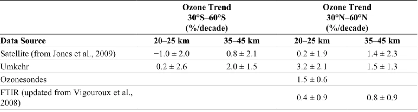
Jones et al. (2009) provide a global estimate of ozone trends from the average of various satellite ozone anomaly records. Using the PWLT statistical model with a turning point in 1997, they find that the largest statistically significant ozone declines in 1979–1997 are found in the midlatitude regions between 35 and 45 km altitude in both hemispheres, with trend values of approximately −7%/ decade. For the period 1997 to 2008, they derive trends of 1.4 and 0.8%/decade in the NH and SH respectively, but these are not statistically significant (see Table 2-2).
Ozone Changes in the Lower Stratosphere
The lower stratosphere between 20 and 25 km over middle latitudes is another region where a statistically sig-nificant decline of about 4 to 5%/decade (or 7–8% total de-cline) occurred between 1979 and the mid-1990s, followed by stabilization or a slight (2–3%) ozone increase thereafter.
Angell and Free (2009) analyzed long-term ozone profile time series from four Northern Hemisphere Dobson Umkehr and 9 ozonesonde stations for trend analysis be-tween 1970 and 2007. The 5-year trends were derived
from the 11-year running mean of the time series to mini-mize the impact of the 11-year solar cycle and QBO sig-nals in the data. Both Umkehr and sonde data showed that nearly half of the increase in north temperate total-ozone trend between 1989 and 2000 was due to an increase in the 10–19 km layer in the lower stratosphere, with the tropo-sphere contributing only about 5% of the change. Nonsig-nificant positive ozone trends at the end of the record in 2000 were found at four Umkehr layers in the middle and high stratosphere, as well as between 10 and 32 km altitude in sonde data.
Murata et al. (2009) could not detect any trend from a 14-year data set of ozone profiles measured with a bal-loonborne optical ozone sensor beginning in 1994 at Sanriku, Japan. This lack of trend was attributed to the leveling off of ODSs in the stratosphere. The extension of the FTIR trend analysis up to 2009 shows no significant trend at the midlatitudes station for the 18–27 km layer (Table 2-1). Similarly, the global trend analysis of Jones et al. (2009) shows no significant trend for the 20–25 km altitude range in the NH and SH midlatitudes for the period 1997–2008.
Figures 2-6a and 2-6b show the temporal evolution of deseasonalized ozone monthly means in three pressure ranges (upper, lower and lowermost stratosphere) based on ozonesondes, Umkehr, and SBUV(/2) observations over Europe and Lauder in the SH respectively (adapted from Terao and Logan, 2007). The various time series show very similar interannual variation, although some biases are apparent between the measurements. In the up-per and lower stratosphere, ozone levels have stabilized after a decrease from the early 1980s to the mid-1990s. In the lower stratosphere, the decrease was more pronounced over Europe than in the SH. In the lowermost strato-sphere, no significant long-term variation is observed at
Table 2-2. Average ozone trends and uncertainties (95% confidence limits) in %/decade in the lower and upper stratosphere in the NH and SH midlatitudes, from various data sources for the period 1996–2008.
The ozonesondes and Umkehr results correspond to the PWLT trends in Figure 2-7. The FTIR results are for the Hohenpeissenberg station only and correspond to the 27–42 km altitude range for the upper stratosphere.
Ozone Trend 30°S–60°S (%/decade) Ozone Trend 30°N–60°N (%/decade) Data Source 20–25 km 35–45 km 20–25 km 35–45 km
Satellite (from Jones et al., 2009) −1.0 ± 2.0 0.8 ± 2.1 0.2 ± 1.9 1.4 ± 2.3
Umkehr 0.2 ± 2.6 2.0 ± 1.5 3.2 ± 2.1 1.5 ± 1.3
Ozonesondes 1.5 ± 0.6
FTIR (updated from Vigouroux et al.,
1.6−6.4 hPa
Smoothed Deseasonalized Monthly Means
−10 −5 0 5 10−63 hPa −40 −20 0 20 Sondes SBUV Umkehr 100−250 hPa −40 −20 0 20 Year
Ozone Anomaly (DU)
(a) Europe
1980 1985 1990 1995 2000 2005 2010
1.6−6.4 hPa
Smoothed Deseasonalized Monthly Means
−10 −5 0 5 10−63 hPa −40 −20 0 20 Sondes SBUV Umkehr 100−250 hPa −40 −20 0 20 Year
Ozone Anomaly (DU)
1980 1985 1990 1995 2000 2005 2010
(b) Lauder
Figure 2-6. (a) Monthly ozone
anoma-lies in Dobson units for Europe as mea-sured by ozonesondes (black line), SBUV(/2) (red line), and Umkehr (blue line) at three pressure layers. The monthly anomalies were computed as the difference between a given monthly mean and the average of monthly means for 1979–1987 for each data set. The average of the monthly-mean anomalies for 1979–1981 was then subtracted from each anomaly time se-ries to set the zero level in each panel. A three-month running mean was ap-plied to the anomalies. The SBUV(/2) data were selected within a grid box of 45°N–55°N and 10°W–30°E. The ozonesonde data are the average of measurements at three European sta-tions: Hohenpeissenberg, Payerne, and Uccle. The Umkehr data are from Arosa, Belsk, and Haute-Provence Observatory. The sonde and SBUV(/2) analysis is updated from Terao and Logan (2007). (b) Same as for (a) but for the Southern Hemisphere. The sonde data are from Lauder, New Zealand. The SBUV(/2) data were se-lected within a grid box of 40°S–50°S and 150°E–170°W. The monthly ano-malies were computed using the monthly means for 1987–1991.
either location over the whole period, but higher short-term variability was seen during the nineties in Europe.
The vertical profile of ozone trends computed from SBUV(/2), Umkehr, and ozonesonde data over Northern midlatitudes stations is displayed in Figure 2-7 for both the increasing and decreasing periods of EESC (e.g., 1979– 1995 and 1996–2008). The trends were derived using EESC as a regression term accounting for the variation of mean age of air as a function of altitude (see Waugh and Hall (2000) for a discussion of age of air and its spatial dependence). In the case of ozonesondes, trends were computed as the average of trends derived for nine northern midlatitude stations, as in the previous Ozone Assessment (Chapter 3). For Umkehr, the trend was derived from the average of ozone anomalies at four northern midlatitude stations and for SBUV(/2), the 40°N–50°N zonal mean data were used. Piecewise linear trends with inflection
point in January 1996 derived from ozonesonde and Umekhr data are also represented in the figure. As shown in WMO (2007), ozone trends during the first increasing period of EESC display two maxima in the upper and lower stratosphere, reaching −5 to −7%/decade and −4 to −5%/ decade respectively (total decline of about 10% and 7% respectively), with generally good agreement between the various observations, except for Umkehr in the lower stratosphere. In both cases, the EESC and PWLT trend models give similar results for this period. For the decreas-ing EESC period, positive ozone trends are derived. In the upper and lower stratosphere, EESC and PWLT models provide similar trends of about 2%/decade. The PWLT trends are significant in the lower stratosphere and barely significant in the upper stratosphere. These results indicate that while the decrease of ODSs is indeed causing an increase of ozone over these midlatitude stations, this
in-−10 −5 0 5 10 1 10 100 400 200 40 20 4 2 0.4 0.2 Pressure (hPa ) Trend (%/decade) 1979−1995 −10 −5 0 5 10 10 14 18 22 26 30 34 38 42 46 50 54 58 62 Altitude (km) EESC SBUV EESC Umkehr PW Umkehr EESC sondes PW sondes −10 −5 0 5 10 1 10 100 400 200 40 20 4 2 0.4 0.2 Pressure (hPa ) Trend (%/decade) 1996−2008 −10 −5 0 5 10 10 14 18 22 26 30 34 38 42 46 50 54 58 62 Altitude (km) EESC SBUV EESC Umkehr PW Umkehr EESC sondes PW sondes (b) (a)
Figure 2-7. Vertical profile of ozone trends over Northern midlatitudes estimated from ozonesondes, Umkehr,
and SBUV(/2) measurements for the period 1979–2008. The trends were estimated using regression to an EESC curve and converted to % per decade using the variation of EESC with time from 1979 to 1995 in panel (a) and from 1996 to 2008 in panel (b). Piecewise linear trends with inflexion point in January 1996 derived from ozonesonde and Umkehr data are also shown. The trend models also include QBO and solar cycle terms. The sonde results are an average of trends for Churchill, Goose Bay, Boulder, Wallops Island, Hohenpeissenberg, Payerne, Uccle, Sapporo, and Tateno, along with two standard errors of the nine trends. The Umkehr trends were derived from averaged ozone anomalies at Belsk, Arosa, OHP, and Boulder. For SBUV(/2), the 40°N– 50°N zonal mean data were used. The altitude scale is from the standard atmosphere. The error bars corres-pond to 95% confidence interval.
crease is still barely significant, especially in the upper stratosphere where trends derived from PWLT and EESC models are expected to show the best agreement. In con-trast, in the lowermost stratosphere, EESC and PWLT trends derived from sondes data differ significantly, with large positive trend values in the latter case, suggesting that the ozone increase is due to factors other than chlorine de-cline, for example dynamical processes (see Section 2.4).
Table 2-2 summarizes the average trends found from various data sources using the PWLT model in the NH and SH midlatitudes in the lower (20–25 km) and upper (35–45 km) stratosphere. Most results show posi-tive ozone trends (1–3% increase) since 1996 in the vari-ous regions. These trends are significant at some locations (e.g., over Northern midlatitudes) but the results from global satellite data are still not significant at the 95% confidence level (Jones et al., 2009).
Northern Hemisphere midlatitude (35°N–60°N) ozone between 12 and 15 km decreased by about 9% be-tween 1979 and 1995, and increased by about 6% bebe-tween 1996 and 2009 (Figure 2-7). The increase since the mid-1990s is larger than the changes expected from the decline in ODS abundances.
2.2 POLAR OZONE
Chapter 4 of WMO (2007) (“Polar Ozone: Past and Present”, Newman and Rex et al., 2007) builds upon the sequence of polar ozone chapters in the WMO Assessment series. The present discussion updates WMO (2007), highlighting changes over the past four years. Discussion of polar ozone recovery is found in Chapter 3 of this Assessment, and interactions of polar chemistry and climate are found in Chapter 4.
2.2.1 State of Science in 2006
The discovery of the Antarctic ozone hole by Farman et al. (1985) prompted considerable effort to de-velop the scientific basis necessary to model and predict polar ozone loss. As noted in the previous chapter, the stratospheric chlorine burden reached its peak in the late 1990s and has since begun to decrease. During the period of increasing chlorine concentrations, the springtime po-lar ozone values decreased in both hemispheres. Consis-tently low values in springtime ozone have been observed since the mid-1980s in the Southern Hemisphere. A unique dynamical situation, the first major sudden strato-spheric warming in the Southern Hemisphere, led to the anomalously high ozone levels in 2002; this situation is discussed in detail in Chapter 4 of WMO (2007). The Arctic polar ozone loss is much more variable, depend-ing not just on the stratospheric chlorine level but also on whether or not the winter is cold enough and of sufficient
length for chlorine-catalyzed ozone loss to occur. Because chlorofluorocarbons are long-lived, atmospheric chlorine loading is declining slowly.
The springtime averages of total ozone poleward of 63° latitude in the Arctic and Antarctic are shown in Fig-ure 2-8 (an update of FigFig-ure 4-7 from WMO, 2007). Inter-annual variability in polar stratospheric ozone abundance and chemistry is driven by variability in temperature and transport due to year-to-year differences in dynamics. The horizontal gray lines in Figure 2-8 are the averages of ozone values obtained between 1970 and 1982, and the shading emphasizes the differences between these aver-ages and subsequent years.
WMO (2007) outlined the processes important to polar ozone loss. The rate-limiting step of the domi-nant cycle for polar ozone destruction is the photolysis of chlorine peroxide (ClOOCl, also known as the chlorine monoxide dimer). Since the previous Assessment, a labo-ratory study suggesting a much lower photolysis rate of ClOOCl than previously recommended (Pope et al., 2007) prompted a number of subsequent laboratory studies on the subject. The implications of the laboratory studies since WMO (2007) for the interpretation of the observa-tions of chlorine monoxide (ClO) and ClOOCl and for the assessment of the uncertainty in computation of ozone loss rates are discussed below along with other updates to the photochemical data in Section 2.2.2.
WMO (2007) concluded that Antarctic ozone loss had stabilized over the time period 1995–2005, with high-er ozone levels in 2002 and 2004 that whigh-ere dynamically
63o-90o Total Ozone Average
1970 1980 1990 2000 2010 Year 200 250 300 350 400 450 500
Total Ozone (DU) BUV EPTOMS_V8C METEOR3_V8 NIMBUS7_V8 OMI_V8F Merged SH October NH March
Figure 2-8. Total ozone average (Dobson units) of
63°–90° latitude in March (NH) and October (SH). Symbols indicate the satellite data that have been used in different years. The horizontal gray lines rep-resent the average total ozone for the years prior to 1983 in March for the NH and in October in the SH. Updated from Figure 4-7, WMO (2007).
driven and not related to reductions in the stratospheric halogen load. For the Arctic it was concluded that for the coldest Arctic winters, the volume of air cold enough to support polar stratospheric clouds (PSCs) had increased significantly since the late 1960s. Arctic spring total ozone was reported to be lower than in the 1980s and was also noted to be highly variable from year to year depend-ing on dynamical conditions. This is discussed further in Sections 2.2.4 and 2.2.5.
Transport and mixing both affect high-latitude win-ter ozone, making it challenging to diagnose the chemi-cal loss rate from observations. WMO (2003) presented an overview of various methods that have been used to separate these effects, mainly for the Arctic winter. WMO (2007) included a comparison of the methods, focusing on the 2002/2003 winter. This colder-than-average winter was chosen because aircraft and ground field campaigns provided the data needed to assess our understanding of polar ozone loss, particularly for the large solar zenith angle-conditions of early winter. WMO (2007) noted that the various methods had been refined since WMO (2003) and produced consistent results.
WMO (2007) included evidence that nitric acid tri-hydrate (NAT) polar stratospheric cloud particles nucleate above the ice frost point and are widespread. Improved NAT mechanisms in chemistry-transport models (CTMs) produce more realistic denitrification, but fail to capture observed interannual variability for the northern winters. Issues concerning polar stratospheric clouds and their representation in models are discussed in Section 2.2.3. This section emphasizes new measurements from the Cloud-Aerosol Lidar and Infrared Pathfinder Satellite Observation (CALIPSO) satellite launched in 2006.
2.2.2 Polar Ozone Chemistry
Chemical loss of polar ozone during winter and spring occurs primarily by two gas-phase catalytic cycles that involve chlorine oxide radicals (Molina and Molina, 1987) and bromine and chlorine oxides (McElroy et al., 1986).
Cycle 1
ClO + ClO + M → ClOOCl + M (1a) ClOOCl + hν → Cl + ClOO (1b) ClOO + M → Cl + O2 + M (1c)
2 [Cl + O3 → ClO + O2] (1d)
Net: 2O3 → 3O2
Cycle 2
BrO + ClO + hν → Br + Cl + O2 (2a)
Br + O3 → BrO + O2 (2b)
Cl + O3 → ClO + O2 (2c)
Net: 2O3 → 3O2
Loss of ClOOCl by thermal decomposition ClOOCl + M → ClO + ClO + M (1e) or chemical processes that recycle ClO without the forma-tion of O2 do not cause ozone depletion. Production of
Br + OClO by BrO + ClO also leads to a null cycle. Small contributions to polar ozone loss occur due to cycles in-volving the reactions ClO + O and ClO + HO2.
Since WMO (2007), attention has focused on re-solving uncertainties in the photolysis cross sections and quantum yields for the ClO dimer, ClOOCl. Pope et al. (2007) reported a ClOOCl absorption spectrum with cross sections at wavelengths between 300 and 350 nm much lower than recommended and than reported in prior studies (e.g., Sander et al., 2006 (referred to in this chapter as JPL 06-2) and references therein), challenging the fundamental understanding of polar ozone depletion (i.e., Schiermeier, 2007; von Hobe, 2007). Photochemical models using the cross sections reported in Pope et al. (2007), with all other kinetic parameters from JPL 06-2, underestimate the ozone loss rate (von Hobe et al., 2007) as well as observed abundances of ClO (von Hobe et al., 2007; Santee et al., 2008; Schofield et al., 2008). A workshop entitled “The Role of Halogen Chemistry in Polar Stratospheric Ozone Depletion” was convened in summer 2008 to assess the fundamental understanding of polar ozone depletion in light of the Pope et al. (2007) measurements. The fol-lowing material incorporates findings from this workshop (SPARC, 2009).
The small ClOOCl cross sections reported by Pope et al. (2007) have been contradicted by all subsequent laboratory studies, as detailed below. There is now con-sensus in the community that photolysis of ClOOCl occurs much faster than implied by Pope et al. (2007). Further, no credible “missing chemical process” has been pro-posed that can be included in models that use the Pope et al. (2007) cross section values to adequately account for observed levels of [ClO] (or in some cases [ClO] and [ClOOCl]; brackets denote concentration of the species) as well as ozone loss derived from observations. The fundamental understanding that polar ozone depletion is caused primarily by reactions involving ClO + ClO, with significant contribution from reactions involving BrO + ClO, has been strengthened since the WMO (2007), based