Fifth International Conference on Advanced COmputational Methods in ENgineering (ACOMEN 2011) Li`ege, Belgium, 14-17 November 2011 (c)University of Li`ege, 2011
Comparison of Data Transfer Methods between Meshes in the
Frame of the Arbitrary Lagrangian Eulerien Formalism
P. Bussetta1, R. Boman1 and J-P. Ponthot1
1LTAS MN2L, Aerospace & Mechanical Engineering Department B52/3, Universit´e de Li`ege, Chemin des Chevreuils, 1; 4000 Liege, Belgium
e-mails:{P.Bussetta, R. Boman, JP.Ponthot}@ulg.ac.be
Abstract
In nonlinear solid Mechanics, the Arbitrary Lagrangian Eulerian (ALE) formalism is a common way to avoid mesh distortion when very large deformations occur in the modelled process. Usually, the ALE resolution procedure is based on an “operator split”, the second part of which is a Data Transfer between two meshes sharing the same topology (same number of nodes and same number of element neighbours for each of them). Thanks to this interesting property, classical ALE transfer algorithms can be much more optimised in terms of CPU time than the ones that are used in the frame of a complete remeshing. However, the resulting CPU-efficient transfer schemes suffer from two main drawbacks. The first one is a spurious crosswind diffusion coming from the corner fluxes that have been neglected. The second issue is the number of explicit transfer steps which may become very large when the element size decreases. In this paper, these classical ALE Data Transfer methods are compared to more general algorithms which do not make any assumption on the topology of both meshes.
1
Introduction
In the Finite Element Method the quality of the mesh (i.e. weak distortion of the elements) has a great importance in the capacity to solve the problem and in the reliability of the solution. The Arbitrary Lagrangian Eulerian (ALE) formalism can be used to minimize the mesh distortion when very large deformations take place during the computation. Usually, with the ALE formalism, the computation on each time step is divided in two parts: in the first part the classical Lagragian formalism is used to solve the problem. In the second one, the nodes of the mesh are displaced to minimize the element deformations, and the data are transferred from the Lagragian mesh to the Eulerian one. The Projection Operator used to transfer information from between both meshes has a great influence on the quality of the solution. In general, two kinds of fields have to be transferred: the first is defined thanks to the nodal values (primary field) and the second one is defined at the integration points (secondary field). Currently, despite the research effort, no Transfer Method has been recognized as the best. Each method has important disadvantages.
This paper compares the most usual Data Transfer Method (Element Transfer Method [1, 2]) with the Data Transfer Methods based on a Weak Form (using Mortar Element [3, 4] or Finite Volume [5, 6]) and with the ALE Data Transfer Method based on the computation of the flux between the elements (using Finite Volumes [7]).
2
Definition of the Data Transfer Problem
In the case of an ALE problem, the data are transferred from the mesh obtained after the Lagrangian
computation (called old mesh) to the repositioned mesh (called new mesh). Both meshes are composed ofne elements andnn nodes. In the general case, the equilibrium state on the old mesh is defined by
some primary and secondary fields, these ones are needed on the new mesh. The fieldP is known on
the old mesh thanks to the primary fieldPold. The nodal values ofPoldis notedP•old. The value ofP old
on each elementeoldis written as:
Pold= nelem n X j=1 Nj.Pjold (1)
whereNj is the shape function of the nodej in the element eoldandnelemn the number of nodes of the
element. The fieldS is estimated on the old mesh by the secondary field Sold. The value ofSoldon each
elementeoldis defined by means of the values at the integration points (noted•S
old). The nodal values
of the elementeold(notedeS•old) are computed by extrapolation of the values at the integration points of
this element (•Sold). In the general case, these nodal values are different for each element. The fields P and S are evaluated on the new mesh thanks to the primary field Pnewand the secondary fieldSnew, respectively. The aim of Data Transfer Method is to define on the new mesh, the nodal values ofPnew
(P•new) and the values at the integration points ofS new (
•Snew). The properties of the Data Transfer
Method should be a weak numerical diffusion, the conservation of the extrema, and the consistency of data (local equilibrium).
3
Transfer Methods
The Data Transfer Method makes the link between the two discretisations. The reliability of the equi-librium state on the new mesh is directly linked with the Data Transfer Method used.
3.1 Element Transfer Method (ETM)
The Element Transfer Method (ETM) is the most commonly used [1, 2]. The computation of the field on the new mesh is done in two steps:
• Firstly, for each characteristic point (node or integration point) of the new mesh a search is done
to find the element of the old mesheoldin which the characteristic point lies inside.
• Then, the value of the field on this characteristic point is computed by interpolation of the nodal
values of the elementeold. The definition of the value is done for the primary field by the relation:
P•new= nelem n X j=1 Nj.Pjold= Pold(x) (2)
and for the secondary field by:
•S new= nelem n X j=1 Nj.eSjold (3)
The shapes of the elements of the new mesh have no influence of the resulting values of the field. The transfer is done from the old mesh to a characteristic point of the new mesh. On the one hand, for the secondary field, this method does not conserve the extrema because of the extrapolation on the nodal values. On the other hand, the extrema are conserved for the primary field.
3.2 Mortar Element Transfer Method (METM)
The Mortar Element Transfer Method (METM) is based on a weak conservation form of the field (discre-tised by Mortar Elements [3]). The fields on the new mesh are not directly computed at the characteristic points but, it is evaluated considering that the integral of the difference between the value of the fields
on the new mesh and the value on the old mesh is zero ([3, 4, 8]). This integral is done over the new mesh. The value of the primary fieldPnewon the new mesh is computed thanks to the relation:
nnew e X enew=1 Z enew (Pnew− Pold)f de = 0 (4)
and the relation between the secondary fieldSnewandSoldis defined for each elementenewof the new
mesh by:
Z
enew
(Snew− Sold)f de = 0 (5)
wheref is a weighting function defined on each element enew(like a primary field). The nodal value of the functionf , f•could be chosen arbitrarily.
The transfer relation of the primary field (equation (4)) can be written like:
nnew n X A=1 nnew n X B=1 NAB1 PBnew− nold n X C=1 NAC2 PCold fA= 0. (6)
WhereNAB1 andNAC2 are the mortar elements defined as:
NAB1 = nnew e X enew=1 NAB1 (enew); NAC2 = nnew e X enew=1 NA2(enew, NC) (7)
where NC is the shape functions of the node C in the corresponding element eold. NAB1 (enew) and NA2(enew, NC) are the mortar elements linked with the element enew(defined in the relations 9). In the
definition of N1
AB(enew), Ni is the shape function of node i in the element enew. NA2 is the coupling
term between the elementenewand the old mesh.
NAB1 (enew) = Z enew NANB de; NA2(enew, NC) = Z enew NANC de (8)
To compute the integral of the relation (5) the secondary fields are defined on each element eold
(enew), like the primary fields (see equation 1), by interpolation of the extrapolated nodal values.
There-fore, the transfer relation of the secondary field (equation (5)) can be written like:
nnew n X A=1 nnew n X B=1
NAB1 (enew)SBnew− NA2(enew, Sold)
fA= 0. (9)
3.2.1 Evaluation of Mortar Element
The first Mortar Element (NAB1 ) is computed by numerical integration over the element of the new mesh
enew, because it is a product of two shape functions of this element. The evaluation of the coupling term (the second Mortar Element,NA2(enew,•)) is more complex, because, in the general case, the field Sold
is not continuous on each element of the new mesh. In addition, the sum of the shape functionsNColdon each element of the old mesh is not a polynomial function on each element of the new mesh (enew). A numerical and an exact integration are used to compute the Mortar ElementN2
A.
Numerical integration The Mortar ElementNA2 is computed by numerical integration over each el-ement of the new mesh. For the elel-ement of the new mesh enew, the computation is done with nip
integration points. The numerical integration supposes that the value of the field on the old mesh can be evaluated by a polynomial function on each element of the new mesh. However, with the numerical integration, the coupling term (N2
A) only takes into account the element intersections containing at least
Exact integration Each element enew of the new mesh is divided in nsube elements, as each sub-element (esub) is only over one element of the old mesh. So, on each elementesub,NColdis a polynomial function. Finally, the Mortar ElementN2
Ais computed exactly by numerical integration over each
sub-elementesub. The exact integration of Mortar Elements considers all intersections between the elements of the new mesh and the elements of the old mesh.
3.2.2 Evaluation of a field on the new mesh
Global solving (GS) The relation between the nodal value of the fieldSnew on each element of the new mesh and the value of the fieldSold(equation (10)) can be written as:
N111 (enew) · · · N 1 1nelem n (e new) .. . . .. ... Nn1elem n 1(e new) · · · N1 nelem n nelemn (e new) S1new .. . Snnewelem n = N12(enew, Sold) .. . N2 nelem n (e new, Sold) (10)
The size of this system of equations is equal to the number of nodes of the element of the new mesh. The value at each integration point is equal to the interpolation of the nodal values. This system of equations can be solved for each element of the new mesh.
For the primary field, equation (6) can be written as:
N111 · · · N 1 1nnew n .. . . .. ... Nn1new n 1 · · · N 1 nnew n nnewn T1new .. . Tnnewnew n = Pnold C=1N 2 1CTCold .. . Pnoldn C=1N 2 nnew n CT old C (11)
The size of this system is equal to the number of nodes of the new mesh. In addition, the solution of this equation cannot guarantee the conservation of the extrema.
Local solving (LS) To obtain a local system, a diagonal matrix is used. The value of the diagonal term is equal to the sum of the line (or the column, because the matrix is symmetric). This is totally equivalent to the row-sum technique used to lump the mass matrix in an explicit time integration method.
So the value of the fieldS on each node of the element enewis done by:
SAnew= N 2 A(enew, Sold) Pnelemn B=1 N 1 AB(enew) (12)
The value at each integration point of the elementenewis computed by interpolation of the nodal values. And, the value of the fieldP on each node is evaluated by:
PAnew= Pnoldn C=1N 2 ACPCold Pnnewn B=1 N 1 AB (13) With this method, a weak conservation of the field is verified in a cell composed of the elements of the new mesh including the nodeA. This technique increases the area of computation of a nodal value and
in the same time the numerical diffusion. But, in opposition of the global solving, the local solving conserves the extrema.
To sum up, the computation of the field is done at the node of the new mesh thanks to the shape function of the elements of the new mesh and the value of the field on the elements of the old mesh.
3.3 Finite Volume Transfer Method (FVTM)
With the Finite Volume Transfer Method (FVTM), each field is rebuilt thanks to an auxiliary mesh (called old finite volume mesh on the old finite element mesh and new finite volume mesh on the new finite element mesh). The finite volumes are called cells. For the primary field, one cell is built on each node of the finite elements mesh. The boundary of this cell is composed of the lines linking the centre of the neighbour finite element to the middle of the edge lied to this node (see figure 1). For the secondary field know thanks tonipintegration points, each element of the finite element mesh is divided in nip
cells (one cell by integration point: see figure 1). So, each field is transferred from one old finite volume mesh to a new finite volume mesh. The same procedure is used to transfer the primary and the secondary field (to more information on the reconstruction of the field see [7, 9]).
Figure 1: Finite element mesh and finite volume mesh based on integration points and on the nodes
3.3.1 Field reconstruction
Constant reconstruction (CR) The value of the field ϕnew (primary or secondary) on one cell is
constant and equal to the value of the field at the corresponding characteristic point (node or integration point) of the finite element mesh.
Linear reconstruction (lR) The value of the fieldϕnew(primary or secondary) on one cell is defined
by a spatial linear function. The value of this field is defined thanks to a mean value and a spatial gradient. The mean value corresponds to the value on the constant rebuilding (the value at the characteristic point). The gradient is defined like the value on the boundary of this cell is always between the main value of this cell and the main value of the neighbour cell (to more information see [7]).
3.3.2 Evaluation of the field on the new mesh
The equation used to evaluate the value of the fields is the same that used with the Mortar Element Transfer Method (see equations 4 or 5). Nevertheless, the functionf is constant on each cell. So, the
mean value of the fieldϕnewon one cellcnewof the new finite volume mesh (ϕnew• ) is obtained with: ϕnewcnew = R cnewϕolddc Vnew c . (14)
Whereϕoldis the value of the field on the old finite volume mesh. Like in the Mortar Element Method, a numerical or an exact integration can be used to evaluate the coupling between the cells of the old and the new mesh.
Numerical integration The value of the fieldϕnewon the cellcnewis defined by numerical integration over this cell. This computation supposes that the field on the old finite volume mesh can be evaluated by a polynomial function on this cell.
Exact integration A super-mesh is built, each cellcnewof the new mesh is divided innc
subcells, like
each of them corresponds only to one cell of the old mesh. For each cell cnew the value ofϕnewcnew is
computed by:
ϕnewcnew =
Pncsub
csub=1 R
csubϕoldcsub dc
Vnew c
. (15)
Where ϕoldcold is the value of the cell of the old mesh corresponding to the sub-cell csub. The exact
integration of coupling considers all intersections between the cell of the new mesh and the cells of the old mesh.
3.4 Convection Transfer Method (CTM)
In the ALE formalism, the number of nodes and finite elements of the mesh as well as their connectivities do not change throughout the simulation. Consequently, the previous general method (FVTM) involving arbitrary meshes may be greatly simplified by avoiding the costly search operation of mesh intersections. Indeed, if the displacements of the nodes are relatively small during the node relocation step, the sum over the sub-cells in Equation (16) may be approximated by :
ϕnewcnew = 1 Vnew c nc sub X csub=1 Vcsubϕ old csub ≃ 1 Vnew c Vcoldϕ old cold− nb,c X j=1 ∆ϕj,c (16)
wherenb,cis the number of boundaries (edges in 2D or facets in 3D) of cellc. The new term∆ϕj,cis an
integral of the reconstructed fieldϕoldover the volume that is swept by the boundaryj of cell c during
the relocation step. This integral may be interpreted as the convective flux ofϕ leaving the cell c during
the definition of the new mesh. It is easily computed by :
∆ϕj,c = Z
∆Vj
ϕold(x) dV (17)
By convention, ∆Vj is positive for an outward flux. Figure 2 geometrically compares the exact
evaluation of a single term of Equation (16) in the case of the FVTM and the approximated flux which is used in the CTM. The difference between both values is usually called corner flux since it directly results from the missing terms related to the neighbours that share a corner with the considered cell.
Vnew c Vnew c corner flux exact (FVTM) approximated (CTM)
flux recieved from the left cell
DVci
Vcsub
Figure 2: Exact and approximated evaluation of the terms of Equation (16).
It can be shown that this simplified scheme is stable if the sum of the swept volumes related to inward fluxes is smaller than the volume of the cell in the new mesh :
X
∆Vj<0
For a uniform one-dimensional mesh, it means that the node displacement during the relocation step should never exceed the length of the cells. In practice, if this stability condition is not satisfied, the total displacement is divided into several convective steps.
4
Numerical examples
The difference between these Data Transfer Methods is shown on two-dimensional academic examples computed with theALEformalism. The first one exposes the numerical diffusion. The second example is a thermo-mechanical problem. The meshes are composed of quadrangular elements. The evaluation of the Mortar ElementN1
AB is done by numerical integration using two Gauss points in each direction.
For the numerical integration, the coupling elements (Mortar ElementNAC2 or coupling between cells) are evaluated with five Gauss points in each direction. For the exact integration, the evaluation of the coupling elements is done using six Gauss points on each triangle of the subdivision (to exact integration of quadratic function).
4.1 Numerical diffusion
The numerical diffusion related to the Data Transfer Operator is studied with this example. A square of sideL is displaced on this diagonal direction. The square’s sides are meshed by 10 elements. The initial
value of all fields is zero. The value for each point of the new mesh which is outside of the old mesh is equal to one on one side of the diagonal and zero on the other one. The total displacement corresponds to the value of the square’s diagonal and it is dived in 20 steps. After each step, the transfer of the primary and the secondary fields is done from the displaced mesh to the initial mesh.
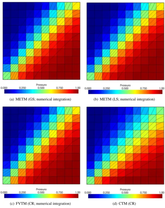
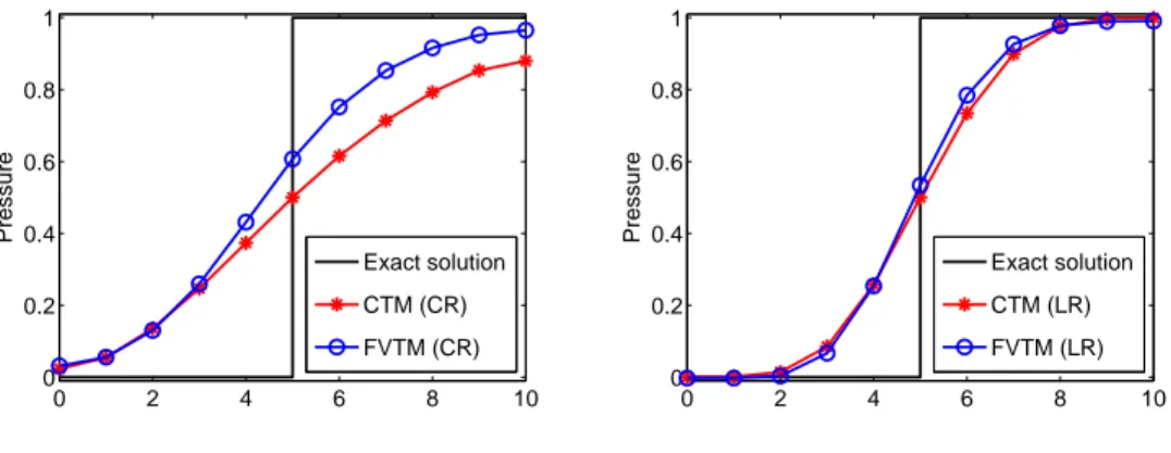
The comparison of the numerical diffusion is done at the end of the simulation (after 20 transfers; see figures 3(a), 3(b), 3(c) and 3(d)). These figures show that the numerical diffusion is more important with the CTM (CR) than with the other Transfer Methods (METM with GS or LS and FVTM with CR). On the other hand, the solution on a line cutting the two opposite square’s sides on their middle is presented at the end of the simulation (see figures 4(a) and 4(b)). These figures illustrate that the numerical diffusion is smaller with the FVTM than with the CTM (with CR as with LR). This difference highlights the influence on the transferred field of the corner fluxes neglected with the CTM. In this case, the difference between the numerical and the exact integration of coupling terms is not significant.
4.2 Necking of a cylinder bar
To compare the presented Transfer Methods, the necking of a cylinder bar is studied. This thermo-mechanical problem is solved in two dimensions with axisymmetric hypothesis and theALEformalism. The length is equal to 53.34 mm and the width is equal to 12.826 mm. Due to the symmetry of the problem, the computation is only done on one quarter of the bar. The mesh of the beam is composed of 28 elements on the length and 16 on the width.
This problem cannot be solved with the ETM because the transfer error prevents the convergence of the next time step. The figures 5 show the value of the equivalent von Mises stress after a lengthening of 16 mm. With the METM with global solving, the difference between the solution and these obtain with the other transfer methods is important. On the other hand, the solution found with the METM with local solving, with the FVTM, or with the CTM is very similar. This example confirm the importance of the Data Transfer Method using in theALE resolution procedure. In this problem, the difference between the solution found with the numerical integration of coupling terms and the one corresponding to the exact integration of coupling terms is small.
(a) METM (GS; numerical integration) (b) METM (LS; numerical integration)
(c) FVTM (CR; numerical integration) (d) CTM (CR)
Figure 3: Numerical diffusion after twenty transfers of the secondary field (1 Gauss points)
5
Conclusion
In conclusion, this paper presents a comparison of Data Transfer Methods in the framework of theALE
formalism. The Data Transfer Methods based on the Weak Form (the Mortar Element Transfer Method and the Finite Volume Transfer Method) are compared to the more used, the Element Transfer Method and the ALE Data Transfer Method based on the computation of the flux between the elements (using
Finite Volumes). With these methods (METM and FVTM) the value of the field at one characteristic point (a node or an integration point) of the new mesh is a function of the value of field on the old mesh and the elements of the new mesh. This paper shows that the transfer error of the FVTM is smaller than the one of CTM, because of the neglected corner fluxes. In addition, the METM with global solving minimizes the numerical diffusion, but the global computation can introduce oscillations around steep variations of the field. So, this method cannot conserve the extrema. On the other hand, the local
0 2 4 6 8 10 0 0.2 0.4 0.6 0.8 1 Pressure Exact solution CTM (CR) FVTM (CR)
(a) With Constant reconstruction
0 2 4 6 8 10 0 0.2 0.4 0.6 0.8 1 Pressure Exact solution CTM (LR) FVTM (LR)
(b) With Linear reconstruction
Figure 4: Numerical diffusion after twenty transfers of the secondary field (1 Gauss point)
a
d
c
b
Figure 5: Value of the equivalent von Mises stress after a lengthening of 16 mm (4 Gauss points): a) METM (GS; numerical integration); b) METM (LS; numerical integration);c) FVTM (CR; numerical integration); d) CTM (CR)
computation increases the smoothing of the field.
point of view of the solution. Nevertheless, The FVTM is more complex, so the CPU times of each transfer is more important. But the FVTM can be used in the general case of the data transfer between different meshes, so no transfer sub-stepping is need in the transfer step of theALEcomputation.
Acknowledgements
The authors wish to acknowledge the Walloon Region for its financial support to the STIRHETAL project (WINNOMAT program, convention number 0716690) in the context of which this work was performed.
References
[1] P.H. Saksono and D. Peri´c. On finite element modelling of surface tension. Comput. Mech., 38:251– 263, 2006.
[2] M. Ortiz and J.J. Quigley. Adaptive mesh refinement in strain localization problems. Computer
Methods in Applied Mechanics and Engineering, 90:781–804, 1991.
[3] D. Dureisseix and H. Bavestrello. Information transfer between incompatible finite element meshes: Application to coupled thermo-viscoelasticity. Comput. Methods Appl. Mech. Engrg., 195:6523– 6541, 2006.
[4] A. Orlando. Analysis of adaptative finite element solutions in elastoplasticity with reference to
transfer operation techniques. PhD thesis, University of Wales, 2002.
[5] A. Orlando and D. Peri´c. Analysis of transfer procedures in elastoplasticity based on the error in the constitutive equations: Theory and numerical illustration. Int. J. Numer. Meth. Engng., 60:1595– 1631, 2004.
[6] F. Alauzet and G. Olivier. An l∞
-lp space-time anisotropic mesh adaptation strategy for time-dependent problems. In Proceedings of the IV European Conference on Computational Mechanics, Paris, France, 16-21 may 2010.
[7] R. Boman. D´eveloppement d’un formalisme Arbitraire Lagrangien Eul´erien tridimensionnel en
dynamique implicite. Application aux op´erations de mise forme. PhD thesis, University of Liege,
2010.
[8] P.E. Farrell, M.D. Piggott, C.C. Pain, G.J. Gorman, and C.R. Wilson. Conservative interpolation between unstructured meshes via supermesh construction. Comput. Methods Appl. Mech. Engrg., 198:2632–2642, 2009.
[9] D.J. Benson. An efficient, accurate, simple ale method for nonlinear finite element programs.