Strategies for Distributed Piezoelectric Actuator / Sensor Placement by Noise Effect Minimisation and Modal Controllability / Observability

Strategies for Distributed Piezoelectric Actuator / Sensor

Placement by Noise Effect Minimisation and Modal

Controllability / Observability

Pascal De Boe(1), Daniel Simon(2), Jean-Claude Golinval(3) LTAS – Vibrations et Identification des Structures,

Université de Liège

Chemin des chevreuils, 1, Bât. B52 B-4000 Liège, Belgium.

e-mail : (1) pdeboe@ulg.ac.be, (2) d.simon@ulg.ac.be, (3) jc.golinval@ulg.ac.be

Abstract

This paper investigates the problem of placement procedure for distributed piezoelectric actuators and sensors. Two placement techniques are proposed. The first one is based on the controllability and observability Grammians of the system expressed in a modal state-space coordinates. The controllability Grammian is then able to quantify how structural modes are controllable with a set of predefined actuators, while the observability Grammian expresses how much structural modes can be observed from a set of predefined sensors. The second placement technique is based on the selection of the best sensor sets which, for each selected structural modes, have the best signal to noise ratio. The sensor selection is performed by inspecting the Fisher information matrix. The number of sensors is then reduced, in an iterative manner, by eliminating locations that do not contribute significantly to the linear independence of the target modal partitions.

Introduction

This paper investigates the problem of placement procedure for distributed piezoelectric actuators and sensors. These last one are very well fitted for applications on plate like structures. The popularity of piezoelectric materials comes from their relative low-cost and light-weight properties and from the fact that piezoelectric laminas can be used as well in actuator mode as in sensor mode.

There exists various attempts to develop a systematic approach for selecting optimal sets of punctual actuators and sensors for experimental identification, but few of them are reported on distributed actuators and sensors.

This problem arises in the case of flexible structure modal identification by means of piezoelectric laminas. An initial mathematical model (generally a finite element model) of the structure is required at the initial step. Assuming that the stiffness and mass influences of the distributed actuators / sensors is negligible in comparison with the support structure, the structural model dynamics (in terms of resonant frequencies and modes) will be independent of the number of candidates for actuator and sensor

locations. This generated model is then used to compute the truncated modal base of the structure in order to retain the more representative set of structural modes.

Two placement techniques are proposed. The first one is based on the controllability and observability Grammians of the system expressed in a modal state-space form. The controllability Grammian is then able to quantify how structural modes are controllable with a set of predefined actuators, while the observability Grammian expresses how much structural modes can be observed from a set of predefined sensors. The procedure begins with the selection of the smallest subset of actuators giving a norm of the system transfer function as close as possible to the norm of the original full set. Once the actuators are selected, the same methodology can be applied to locate the minimum set of sensors.

The second placement technique is based on the selection of the best sensor sets which, for each selected structural modes, have the best signal to noise ratio. The sensor selection is performed by inspecting the Fisher information matrix. The number of sensors is then reduced, in an iterative manner, by eliminating locations that do not

contribute significantly to the linear independence of the target modal partitions contained in the Fisher information matrix.

1. Piezo-structure overview

1.1 Dynamics of piezo-structures

In the case of a structure instrumented with piezoelectric sensor/actuator, electromechanical relationships are added to the dynamics of the system to represent the contributions of the electrical degrees of freedom linked to the piezoelectric actuator and sensor (Saunders et al. [1]) : q v C x v f x K x D x M s p s a a T = ⋅ + ⋅ Θ ⋅ Θ + = ⋅ + ⋅ + ⋅ && & ( 1 ) The first equation is commonly called the actuator equation and the second, the sensor one. The actuator equation exhibits the force generated by the piezoelectric actuator through the electromechanical coupling actuator matrix _Θa _{and the electrical}

potential va applied between the electrodes of the

element. The sensor equation shows the relationship existing between the mechanical degrees of freedom

x and the electrical charges q or potentials vs

through the electromechanical coupling matrix

T

s

Θ and the capacitance Cp of the sensor. When an

external force f acts on the structure, the induced sensor signal depends on the electrical conditions applied at the electrode level :

• Case 1 : open-circuit (q=0)

(

)

0 1 = ⋅ + ⋅ Θ = ⋅ Θ ⋅ ⋅ Θ − + ⋅ + ⋅ − s p s s p s v C x f x C K x D x M T T & && ( 2 )

The corrective stiffness term sT p s C ⋅Θ ⋅ Θ −1 is usally neglected when the partition of piezoelectric elements is small compared to the structure. Thus, the structural dynamics is not modified by the presence of the piezoelectric effect.

• Case 2 : short-circuit (vs =0) q x f x K x D x M T s _{⋅ =} Θ = ⋅ + ⋅ + ⋅&& & ( 3 ) In this case, the capacitance of the sensor is eliminated from the output measurement by means of an appropriate analog circuitry (e.g. : a charge amplifier).

1.2 Sensor and actuator dynamic

reduction

The dynamics of a piezoelectric system described by ( 1 ) is mechanically affected by the presence of the actuator/sensor transducers loading the structure (in terms of stiffness and inertia) : resonance frequencies and mode shapes are theoretically modified by the mechanical characteristics of actuator/sensor. If the transducer placement strategy consists of a computation of a position index performance, it induces that the eigen-value problem has to be solved at each iteration. This is very costly and becomes prohibitive in case of large structures.

Therefore, when the partition of distributed transducers is negligible compared to the main structure, one will neglect the inertia associated with the transducers (weight of piezos << structural weight) as well as their stiffness (local stiffening neglected); only the electromechanical coupling will be taken into account. As an example, let us take a structure fitted with two decoupled piezo-laminates. Figure 1(a) shows the global stiffness connectivity of the initial system :

                Θ Θ s p a p T s a s a s struct a struct struct C C K K K K K O O O O O O O O O 0 0 0 0 0 0 / / ( 4 )

where mechanical and electrical degrees of freedom (d.o.f.) are organised in such a way that :

{

}

T s a s a struct x x v q x ( 5 )

with xstruct, the d.o.f.’s of the main structure and xa, s

x are related to the actuator and sensor mechanical d.o.f.’s.

When performing the finite element model (FEM) of the distributed transducers, a reduction of transducer degrees of freedom (d.o.f.) (e.g. : using Guyans’s reduction technique [2]) can then be performed as follows :

• Modelling of the distributed transducers.

• Reduction of the system to the structural interface degrees of freedom.

• Setting of the resulting transducer mass and stiffness matrix to zero (inertia and stiffening neglected).

• Assembling of the modified transducer model with the main structure.

The resulting system has only the following d.o.f. :

{

}

T s a struct v q x ( 6 )

and figure 1(b) shows the connectivity of the resulting reduced system.

When the partition of piezoelectric elements is small compared to the main structure, reduction errors on resonance frequencies and mode shapes are small, leading to an acceptable model for applying actuator / sensor placement techniques. In the following transducer models will be used in the condensed form.

(a) (b)

Figure 1 : Connectivity of a piezo-structure (a) full system, (b) condensed system

2. The modal approach of

controllability and observability

2.1 State-space modal representation

To apply the theory of controllability and observability, which has been developed in the theory of control, it is convenient to express the system nodal representation in the generalised form : x C x C y u B x K x D x M x x & & && &⋅ + ⋅ = ⋅ = ⋅ + ⋅ + ⋅ 0 0 0 ( 7 ) where y is defined as the output vector and depends linearly of the structural displacements and velocities. Defining the state variables as the modal displacement and velocities :

      = m m m x x X & ( 8 )

the modal state-space representation takes the form :

m m m X C y f B X A X & & ⋅ = ⋅ + ⋅ = _{( 9 )}

with the following triplet :

[

mx mx

]

m C C C B B Z I A _ = _&      =       Ω − Ω − = , 0 , . . 2 0 2 ( 10 )

where Ω=diag(ω1,ω2,Kωn) is the spectral matrix associated with the

(

n×nm

)

modal matrix

[

φ1 φ2 K φnm

]

=

Φ . The modal mass, damping (assumed proportional) and stiffness matrix are obtained by the modal projection of K, D, M :

1 1 . . . 2 1 , . . . . , . . − − _Ω = Φ Φ = Φ Φ = Φ Φ = m m T m T m T m D M Z K K D D M M ( 11 )

In the same way, the modal input, displacement and velocity output matrices are introduced by :

Φ = Φ = Φ = −_{. . , . , .} 0 0 0 1 x x m x mx T m m M B C C C C B _{& &} ( 12 )

By simply rearranging the lines of ( 8 ) in order to organise the state components as follows :

{

}

T x x x x m m mn n m m m1 & 1 K & ( 13 )

the modal state-space representation is characterised by a block diagonal structure :

[

m

]

m mn m mn m mi C C C B B B A diag A M 1 L 1 , ), ( =           = = ( 14 )

The dimensions of this modal state-space representation

(

2⋅nm×2⋅nm

)

are then more

economic than the nodal representation

(

n×n

)

since

n nm<< ⋅

2 for a modal truncated system.

2.2 Controllability and observability

In classical control theory, a linear time invariant system

(

A,B,C

)

is fully controllable if and only if the constructed matrix :

[

B AB A B AN B

]

C

₌ 2 −1

K ( 15 )

has rank N=size

( )

A . In the same way, a linear time invariant system

(

A,B,C

)

is fully observable if and only if the matrix :

            ⋅ ⋅ = −1 N A C A C C O M ( 16 )

has rank N. As clearly explained in Gawronski [6], these criteria, although simple, are not at all efficient :

• the level of controllability or observability is not quantified; these criteria give an answer in terms of yes or no.

• The computation of C or O is prohibitive in the case of system with realistic size.

These two drawbacks bring us to prefer expressing the system properties in terms of Grammians. The controllability and observability Grammians are defined as follows :

( )

( )

t e C C e dt W dt e B B e t W t A t _{A t T} o t A t _{At T} c T T ⋅ ⋅ ⋅ ⋅ ∫ ∫ ⋅ ⋅ ⋅ = ⋅ ⋅ ⋅ = 0 0 _{( 17 )}

The controllability Grammian reflects the ability of a perturbation u to perturb the state of the system. The observality Grammian reflects the ability of a state X to affect the output y of a system. In the case of a time invariant system, the stationary solutions of ( 17 ) are given by the Lyapunov equations : 0 0 = ⋅ + ⋅ + ⋅ = ⋅ + ⋅ + ⋅ C C A W W A B B A W W A T o o T T T c c ( 18 ) The singular values of the Grammians product are invariant under linear transformation and are called the Hankel singular values :

(

Wc Wo

)

i N

i

i = λ ⋅ , =1K

γ ( 19 )

An important advantage of the modal state representation ( 8 ) is that the resulting controllability and observability Grammians are diagonally dominant (see Gawronski [3]) :

) ( ) ( ⋅ 2×2 ≅ ⋅ 2×2 ≅diagw I W diagw I Wc ci o oi ( 20 )

Diagonal entries of ( 20 ) and Hankel singular values could then be obtained as follows :

i i mi mi i i i mi oi i i mi ci C B C w B w ω ζ γ ω ζ ω ζ 4. . . , . . 4 , . . 4 2 2 2 2 2 2 ≅ ≅ ≅ ( 21 )

which is a more efficient way to compute the Gammians than the resolution of equations ( 18 ).

2.3 Transfer function norm

The transfer function of a system, expressed in the state-space form, is given by :

( )

C

(

j I A

)

B

Gω = ⋅ ⋅ω⋅ − −1⋅ ( 22 ) Transfer function norms H2,H∞,HHankel serve as a

measure of the controlling ability of an actuator / sensor configuration applied on a system

defined by

(

A,B,C

)

. In this paper, only the H2

norm, defined by :

( ) ( )

(

)

(

) (

o

)

T c T W B B tr W C C tr d G G tr G ⋅ ⋅ = ⋅ ⋅ = ⋅ ⋅ ⋅ =

_∫

₋+_∞∞ ω ω ω π * 2 ₂ 1 ( 23 )

will be considered. The second part of ( 23 ) shows the cross-connectivity between the output matrix C

and the observability Grammian WC (and

vice-versa) on the system norm.

For flexible systems in the modal state representation, H2 norm can be expressed in terms

of the norms of the modes. This modal decomposition affords then a visibility on each modal contribution. Taking the transfer function of the ith mode :

( )

mi

(

mi

)

mi

i C j I A B

G ω = ⋅ ⋅ω⋅ − −1⋅ ( 24 ) the H2 norm of the i

th

mode can be estimated (see Gawronski [6]) by : i i i mi mi i i mi mi i C B C B G ω γ ω ω ζ ∆ ⋅ ⋅ ≅ ∆ ⋅ = ⋅ ⋅ ⋅ ≅ 2 2 2 2 2 2 2 _{( 25 )}

where ∆ωi =2⋅ζi⋅ωi is the half-power frequency at

the ith resonance. By using ( 23 ) and since the Grammians are diagonally dominant in the modal state-space representation, the H2 norm of the

complete system is estimated by the rms sum of the modal norms :

∑

= = nmt i i G G 1 2 2 2 ( 26 )

where nm_t (<<nm) is the number of targeted modes.

Equations ( 25 ) and ( 26 ) are the bases for actuator and sensor placement strategies.

2.4 Placement strategy for structural

testing

This technique addresses the problem of targeted mode identification in structural testing. The aim is to select a minimal number of actuators and sensors that would measure, as accurate as possible, targeted modes. For a realistic structure, the procedure has to take into account geometrical constraints that limits the number of candidate locations.

2.4.1 Actuator positioning

Assuming that sensors are placed at all candidate locations (C is then fixed for comparison purpose only), the principle of the method is to compute, for each possible actuator locations, the placement index σ2ki that evaluates the importance of the k

th

(

1Kna<n

)

actuator at the i th

(

)

t m n K 1 mode to the performance achievable with the full set of actuators (we cannot afford the full set of actuators, and it will used for comparison purpose only) :

2 2 2 G G wki ki ki = ⋅ σ ( 27 )

where wki is an user defined weighting coefficient

that reflects the importance of the ith mode and the kth actuator in the application. A placement matrix can then be constructed by varying B0,C being

fixed : actuator k mode th 2 1 2 21 211 2 ⇑ ⇐           = Σ th n n n n a i a t m t m a σ σ σ σ L M O M L ( 28 )

Each terms of ∑2 show the ability of the k

th

actuator position to affect the ith mode. The actuator index, computed by the rms sum of the kth actuator over all the modes :

∑

= = nmt i ik a k 1 2 σ σ ( 29 )

reflects an averaged ability of the kth position to affect all the targeted modes.

In the case of a large (and complex) structure, the maximisation of a

k

σ alone is not a satisfactory criterion : too many locations have to be selected to guarantee a sufficient excitation of all the targeted modes. On the other way, a strategy based on the selection of the s1 higher placements for each mode

will give too many locations with comparable efficiencies [3]. These locations can be extracted using an additional criterion based on the correlation of each actuator modal norm vector :

              = 2 2 2 2 2 2 2 1 t m kn k k k G G G g M ( 30 )

with Gki ₂, the H2 norm of the transfer function of

the kth candidate actuator on the ith targeted mode. An assurance criterion (AC) is then used to distinct high correlated actuator candidate locations :

(

,

)

1 0 2 2 ≤ ⋅ ⋅ = ≤ l k l T k l k g g g g g g AC ( 31 )

When AC

(

gk,gl

)

≥1−ε (with ε , a small positive number), it means that these two actuator candidate locations will excite the targeted modes with an equivalent efficiency; one of these two candidates can then be removed.

Based on the above analysis, the actuator placement strategy is established :

1) Construct the actuator placement matrix a

2

∑ . 2) For each targeted mode, select the sm most

efficient locations. The resulting number of actuators s1 is then much smaller than the number

of candidate locations : a m m n n s s t << ⋅ ≤ 1

3) Check the correlation between the remaining actuator modal norm vector gk, keep all

non-correlated locations with AC

(

gk,gl

)

<1−ε and keep also the one with the higher index a

k

σ for correlated actuators. The number of remaining locations is now s2<s1<<na.

2.4.2 Sensor positioning

Once the actuator positions are selected (B0 is

optimised), the same procedure can be repeated by constructing a sensor placement matrix that allows the selection of the best sensor positions.

2.4.3 Numerical example

The method for actuator placement strategy, presented in this section, has been applied on a numerical example to locate piezo-laminate for structural characterization. The main structure consists of an 0.16 x 0.08 x 0.001 m clamped-free stainless steel plate (clamped side at x = 0 in figure 3). The problem is to find the minimal set of 0.0508 x 0.0254 x 0.0004 m PZT-laminates able to excite correctly the first five modes of the structure. Structural finite element model

The tested structure is first modelled using the finite element technique. The meshing of the structure is

chosen to be compatible with the piezo elements (see figure 3).

The model uses conventional 3-D isoparametric solid elements, improved by adding incompatible second order shape functions associated to nodeless degrees of freedom. This technique has been introduced by Bathe and Wilson [4] and applied to piezoelectric structure by Tzou and Tseng [5]. The resulting model totalises 918 mechanical d.o.f.’s. Table 1 gives the computed resonance frequencies associated with the five first modes of the tested structure.

Hz Shape Mode 1 27.9 (11) Mode 2 134.3 (12) Mode 3 165.8 (21) Mode 4 442.7 (22) Mode 5 473.2 (31)

Table 1 : Eigen-frequencies of tested structure Actuator placement procedure

Due to obvious physical constraints, only 91 candidate actuators have been identified :

• 7 positions along the y axis

• 13 positions along the x axis.

Assuming that only vertical displacements (z direction) are monitored :

0 , 0 =

= z x

ox I C

C & ( 32 )

the actuator placement matrix a

2 ∑ is constructed by setting, in ( 7 ) : a k k B0 =−Θ ( 33 ) where a k

Θ is the electromechanical coupling of an actuator at the kth position.

Figure 2 : Actuator modal performances

Results

The procedure described in § 2.4.1 is then applied and leads to the actuator placement matrix shown in figure 2. Note that the actuator controllability on the mode 1 (flexion along the x axis) is logically decreasing with the distance between actuator and the clamped side of the plate.

The three remaining actuator locations (on 91 candidates!) are presented in figure 3. By checking the actuator modal performance matrix, it is interesting to note that the actuator location n°1 has a good efficiency to excite the 3 first modes while position n°35 and n°57 have been selected to excite modes 4 and 5 respectively.

Figure 3 : Controllability placement procedure results.

3. Sensor placement technique

based on noise minimisation

effect

For practical reasons it is of course impossible to make measurements at all structural degrees of freedom. The position and number of sensors not only condition the modal extraction, but also the resulting spatial independency of the modal base formed by the *

s

n sensors on thenm_t targeted modes.

Spatial independency is important when the experimental identification goal is to serve as input for, e.g. a model updating procedure : a linear dependency between extracted modes leads to ill-posed problems because it will be impossible to distinguish modes from each other. Kammer [6] has proposed an iterative method that selects measurement locations, assuring that the measured modal base will be linearly independent.

(0, 0, 0) x y z N°1 N°57 N°35

3.1 Placement procedure

Spatial independency implies that the estimate qˆ of the target modal coordinates q is found in a least squares sense :

[

]

s T s s T s u qˆ= Φ ⋅Φ −1⋅Φ ⋅ ( 34 ) with us =Φs⋅q, the sensor outputs,

s

Φ , the nm_t targeted modes given at all sensor

candidates.

Let us assume that the sensor outputs are polluted by a stationary Gaussian noise, uncorrelated and with equivalent statistical properties for each sensor. The variance is given by :

( )

n n I

E _⋅ T ₌ 2_⋅

0

ϕ ( 35 )

The criterion to choose the location of the sensors is given by the minimization of the covariance matrix for the estimates of the modal displacements :

( ) ( )

[

T

]

q q q q E ˆ ˆ min − ⋅ − ( 36 )

This problem is equivalent to maximize the Fisher information matrix expressed by :

(

)

2 0 0 1 2 0 max max ϕ ϕ s A T s⋅Φ = Φ ⋅ − ( 37 ) Equation ( 37 ) implies then that the signal to noise ratio is maximised.

For convenience, the trace will be used as the matrix norm :

( ) ( )

= Λ =tr A tr

A0 0 ( 38 )

where Λ comes from the associated eigenvalue problem : Λ ⋅ Ψ = Ψ ⋅ 0 A ( 39 )

The degrees of freedom not contributing to the norm of A0 do not affect the estimation of the

modal components and their measurement is useless. Let us define a scaled matrix in wich each row contains the square of the components of the rows of Φs in terms of the basis Ψ :

[

] [

]

(

_{Φ ⋅Ψ ⊗Φ ⋅Ψ}

)

_⋅Λ−1

= s s

E

F ( 40 )

where ⊗ indicates a term by term product.

The sum of the elements of each row (the row number corresponding to a sensor candidate) of FE

is a measure of its contribution to Λ. The effective independence of a sensor can then been checked at

each iteration, the location showing the lowest sum value is then removed from the list.

To prevent rank deficiency of A0 (and by the way,

to allow the computation of qˆ in ( 34 )), the iteration procedure is stopped when the number of retained locations is equal to the number of targeted modes. The derived sensor configuration is said suboptimal because it is generated in an iterative manner.

3.2 Numerical example

The same set-up, as described in §2.4.3 is used. The final goal is, this time, to find the minimal sensor set able to identify the first 5 modes of the structure. To adapt Kammer's algorithm for distributed sensors, the procedure starts from the computation of the piezoelectric output modal base, where each component is the response of each candidate sensor to a modal structural deformation :

[

]

i T s n s k s piezo i _s φ φ = Θ1 L Θ L Θ ⋅ ( 41 ) with s k

Θ is the electromechanical coupling of the kth distributed sensor candidate,

i

φ is the ith targeted mechanical mode.

piezo i

φ is the ith mode expressed in the distributed sensor coordinates.

Figure 4 presents the achieved effective independence distribution defined by :

( )

∑

= =nmt i E i F EfI 1 :, ( 42 )

for all iterations.

Figure 4 : EfI distribution for all iterations. The trace of the Fisher information matrix is also presented in figure 5. Its value is logically decreasing as the number of sensors decreases, but is maintained to an acceptable value in order to achieve a sufficient signal to noise ratio.

Figure 5 : A0 trace versus number of sensors.

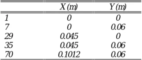
Table 2 gives the reference corner positions of the selected sensors. X (m) Y (m) 1 0 0 7 0 0.06 29 0.045 0 35 0.045 0.06 70 0.1012 0.06

Table 2 : Selected sensor corner positions

4. Conclusion

Placement procedures for distributed transducers have been successfully adapted from existing methods. The first procedure is based on the observability and controllability aspects. The second method, based on the noise minimisation effect can only be applied for sensor placement, but guarantees a linear independence of the resulting sensor base. The two approaches give similar results on simple structure. Nevertheless, the Grammians method is able to take into account the initial sensor and actuator sets : the optimised sensor set will depends on the previously optimised actuator set (and inversely).

Acknowledgements

This work is supported by the Région Wallonne (B) under the contract RW-ULG 9613500.

References

1. Saunders, W.R., Cole, D.G., Robertshaw, H.H., Experiments in piezostructure modal analysis for MIMO feedback control, Smart Mater. Struct., 1994, 3, 210-218.

2. Maia, Silva, He, Lin, Skingle, To, Urgueira, Theoretical and experimental modal analysis,

Research Studies Press LTD., Taunton, England, 1997.

3. Gawronski, W.K., Dynamics and control of structures : a modal approach, Springer-Verlag, New-York, 1998

4. Bathe, K.J., Wilson, E.L., Numerical methods in finite element analysis, Englewood Cliffs, NJ : Prentice Hall, 1976

5. Tzou, H.S., Tseng, C.I., Distributed vibration control and identification of coupled elastic/piezoelectric systems : finite element formulation and applications, Mechanical Systems and Signal Processing, (1991) 5(3), 215-231. 6. Kammer, D.C., Sensor placement for on-orbit modal identification and correlation of large space structures, Journal of G. C. and Dynamics, 14, 251-259.