A robust heuristic for the optimal selection of
a portfolio of stocks
Micha¨
el Schyns
University of Li`ege, HEC-Management School, QuantOM Bd. du Rectorat 7 (B31), 4000 Li`ege, Belgium.
Email: M.Schyns@ulg.ac.be Fax: +3243662767
Abstract: This paper introduces a new optimization heuristic for the robustification of critical inputs under consideration in many problems. It is shown that it allows to improve significantly the quality and the stability of the results for two classical financial problems, i.e. the Markowitz’ portfolio selection problem and the computation of the fi-nancial beta.
Focus here is on the robust Minimum Covariance Determinant (MCD) estimator which can easily be substituted to the classical estimators of location and scatter. By definition, the computation of this estima-tor gives rise to a combinaestima-torial optimization problem. We present a new heuristic, called ’RelaxMCD’, which is based on a relaxation of the problem to the continuous space. The utility of this approach and the performance of our heuristic, with respect to other competitors, are illustrated through extensive simulations.
Keywords: Combinatorial optimization; Robustness; Markowitz’ model; beta computation; MCD estimator.
Reference to this paper should be made as follows: Schyns Micha¨el. (xxxx) ‘A robust heuristic for the optimal selection of a portfolio of stocks’, Int. J. Operational Research, Vol. x, No. x, pp.xxx–xxx.
Biographical Notes: Michael Schyns obtained a PhD in portfolio op-timization from the University of Li`ege in 2001. He is currently Professor of Information Systems at HEC-Management School of the University of Li`ege where he heads the Operations Department. His main research interest is combinatorial optimization applied to management problems and statistics.
1 Introduction
Many financial applications rely on strong assumptions on statistical distribu-tions. Often, critical inputs of financial models are simply the first moments of these distributions. It is well known that the quality of the estimations of these parameters may lead to large variations of the outputs; see e.g. Chopra and Ziemba (1993) or Chen and Zhao (2002) for mean-variance problems. Basic examples in Section 2 show that opposite financial conclusions could be drawn only by
bating one simple historical input. Therefore, since only one gross error in data or one atypical event may lead to the breakdown of the classical mean and covariance estimators, one can wonder whether the results of optimization problems in finance based on these estimators are meaningful. This is the initial motivation of our work: robustify the inputs in order to improve the significance of the outputs; especially in finance.
In this paper, we suggest to turn to robust statistics to compute better estimates of location and scatter. Robust estimators, while usually preserving the basic prop-erties of their classical counterpart, should be able to resist to atypical observations and detect them. We will focus here on the Minimum Covariance Determinant ro-bust estimator introduced by Rousseeuw (1985). Its definition goes as follows. In a sample of n data points, one has to select a subsample of size h≈n
2 minimizing the generalized variance (i.e. the determinant of the covariance matrix based on these points). The location and scatter MCD estimates are then given by the average and covariance matrix of the optimal subsample. The MCD estimator is quite attrac-tive: its definition is simple and intuitively appealing, while it has good theoretical properties (see Butler, Davies and Jhun 1993). However, its computation is hard since the corresponding optimization problem is combinatorial.
The computational complexity of the MCD estimator has given rise to an active research area: Hawkins (1994), Rousseeuw and Van Driessen (1999), Hawkins and Olive (1999), Bernholt and Fisher (2004)... Indeed, an exact computation naively requiring the consideration of all the (nh) subsamples in order to select the best one would be infeasible even for relatively small data sets. Up to now, no exact algorithm is able to deal with real size problems. We have to resort to heuristics. The two most famous ones remain the FASTMCD algorithm of Rousseeuw and Van Driessen (1999) and the Feasible Solution Algorithm of Hawkins (1994), improved by Hawkins and Olive (1999). We however know that the current heuristics usually do not reach the global optimum for most real-size problems and therefore differ-ent approaches, also originating from Operational Research as Branch and Bound, Simulated Annealing, Tabu Search or Neural Networks, have been considered (see e.g. Agull`o 1998, Todorov 1992 and Woodruff 1996). This is the second motiva-tion of our work: develop a more efficient approach and compare it to the main competitors.
The combinatorial definition of the MCD estimator seems to prevent the de-sign of algorithms taking advantage of smoothness properties. Indeed, heuristics presented in the literature are mainly based on classical combinatorial methods. However, the relaxation strategy proposed by Critchley et al (2009) and Schyns et al (2008) allows to transform this discrete and high dimensional optimization prob-lem into a continuous and low dimensional one. Gradient information may then be used to reach an optimum. Based on these papers, a new optimization procedure called ‘RelaxMCD’ is presented and assessed here.
Of course, the reliability of the classical mean and covariance matrix has been under consideration for a long time. A plethora of problems have been attacked and many methods have been attempted. Some of them try to robustify directly the inputs as we do and others work on the whole optimization process (robust op-timization). Among many others see e.g. Fabozzi et al. (2009), Scherer and Martin (2005), Atkinson (2007), Bailer and Martin (2007), Chen and Liu (1993), Delage and Ye (2008), DeMiguel and Nogales (2009), Fabozzi et al. (2007), Garlappi et al.
(2007), Goldfarb and Iyengar (2003), Hubert et al.(2009), Kan and Zhou (2007), Lauprete et al. (2002), Lutgens et al. (2006), Mahaney et al. (2007), Natarajan et al. (2009), Perret-Gentil and Victoria-Feser (2003), Schen and Zhang (2008), T¨ut¨unc¨u and Koenig (2004), Zaman et al. (2001). The reader particularly inter-ested in the robust statistics approach, which can be applied directly to portfolio problems as well as in many other fields, could read recent general introductions as e.g. Maronna et al. (2006), Huber (2009), Hubert et al. (2008) or Ronchetti (2006).
The paper is organized as follow. We first want to show how attractive a robust approach is when considering financial problems. A very basic illustration of the motivation is given in Section 2. Our new algorithm is shortly described in Section 3. The special case of the Markowitz’ problem, whose inputs are mainly estimations of location and scatter of assets returns, will be briefly presented in Section 4. We will also illustrate that all heuristics are not equivalent. The performance of RelaxMCD with respect to the above mentioned competitors for computing MCD and with respect to the classical estimators is measured by means of simulations on real data in Section 5. Conclusions are provided in Section 6.
2 Motivation and basic examples
As explained in the previous section, faithfully computing first and second mo-ments is of capital importance in finance. Unfortunately, the mean and the classical covariance matrix are not robust (see e.g. Donoho and Huber (1983) for a formal definition of the breakdown of these estimators). To illustrate this, let us consider the monthly returns of the S&P500 index over the 5 year period 2003-2007. The classical mean of these 60 observations gives an annualized return of 10%. The computation of the mean was repeated under three different hypotheses. In the first case, the observation corresponding to a huge and atypical decrease (-6.3% in one month) of the index return was deleted. In the second case, we have assumed that the sign of the lowest return was wrong and we corrected it accordingly. Note that this error is not obvious to detect by simple visual inspection since the magni-tude is maintained. Finally, we have assumed that the lowest return was incorrectly encoded and replaced by its percentage value, i.e. multiplied by one hundred. The corresponding annualized mean returns are 8.4%, 12.8% and -70.3% respectively instead of 10.0%. This clearly shows that modifying only one observed monthly return over five years leads to significative variations of the mean value for the investor!
The same can be shown for the covariance matrix. To illustrate this, let us look at the financial beta of a stock. The beta indicates how much the return of a stock (or of a fund) will change, on average, with respect to the market return. A beta of 1.5 means that we can expect an increase (decrease) of 1.5% of the stock return when the market return increases (decreases) by 1%. A beta of 1 implies that the changes in the stock returns are on average of the same amplitude as the market returns. The beta in itself is a useful financial measure of risk. Stocks or funds with beta lower than one, equal to one and larger than one are said to be respectively more agressive than the market, neutral and defensive. It is also used in more advanced models like the Capital Asset Pricing Model (CAPM). It is however well
known in finance that it is dangerous to take decision based solely on the beta for individual stocks. Indeed, it is extremely difficult to obtain the “exact” value (the standard error is typically large) and the beta represents only a link with the market risk but does not integrate the specific risk of the stock (R-squared of the regression is usually considered as low by statisticians). Other questions such as the power of prediction or possible adjustments of the beta are beyond the scope of this section. A more formal introductory description of the financial beta and of the CAPM can be found in Brealey an Myers (2002).
Here, only its mathematical definition is of use to illustrate the lack of robustness of variances and covariances. The beta is simply the slope of the linear regression of the stock returns with respect to the market returns. The beta of a stock i is therefore given by:
βi=
σim
σ2
m
where σimis the covariance between the stock return and the market return and σm2
is the variance of the market returns. These two elements are the main components of the covariance matrix of the market and stock returns that we want to analyze.
−0.26
−0.18
−0.10
−0.02
0.04
0.10
0.16
0.22
0.28
−0.16
−0.08
0.00
0.06
0.12
SP500
EMR
R1: Raw
R2: Exclude X
R3: Sign
R4: %
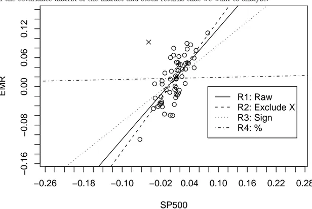
Figure 1 Linear regression of Emerson Electric monthly returns with respect to S&P500 returns
Over the same period 2003-2007, let us focus on the Emerson Electric stock which is a constituent of the S&P500 index. We make the standard assumption that the S&P500 index represents the market and compute the raw beta. Then, similar assumptions as those explained above for the computation of the mean are considered. Results are represented in Figure 1 and in Table 1. We first excluded
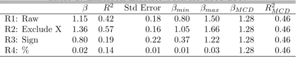
one of the sixty couples of returns which looks atypical (represented by a cross in the figure); the corresponding regression line is given by R2 on the scatter plot. Then we made again the assumption that the sign of the lowest S&P500 return is incorrect (regression line R3) or encoded as a percentage (regression line R4). The first column of Table 1 clearly shows that the beta of the stock is very sensitive to variations in only one observation. According to only this column, we could have three differents conclusions; with respect to the regression R1, the stock is neutral while it is more aggressive with the model R2 and defensive with R3 and R4. However, the standard error on beta, indicated in the third column, is large and no definitive conclusions can be stated. βmin and βmax define the usual 95%
confidence interval for β. Finally, it is interesting to see that the R-squared statistics is reasonnable in the two first lines of the table (especially in the second one where 57% of the total variance of the stock return changes can be explained by the market movements).
Table 1: Emerson Electric beta for 2003-2007
β R2 Std Error β min βmax βM CD R2M CD R1: Raw 1.15 0.42 0.18 0.80 1.50 1.28 0.46 R2: Exclude X 1.36 0.57 0.16 1.05 1.66 1.28 0.46 R3: Sign 0.80 0.19 0.22 0.37 1.22 1.28 0.46 R4: % 0.02 0.14 0.01 0.01 0.03 1.28 0.46
The illustration with the financial beta does not use directly the covariance matrix but a ratio of two of its elements. Statisticians usually illustrate the lack of robustness of the covariance matrix by drawing 95% confidence ellipso¨ıds. The volume and the location of the ellipso¨ıd are fully defined by the covariance matrix and the mean. The main axis of the ellipso¨ıd corresponds to the first principal component. When applied to our data set, we observe cleary the same phenomenon. We have therefore decided to stick to the more applied financial representation.
3 The RelaxMCD heuristic
The definition of the Minimum Covariance Determinant estimator goes as fol-lows. In a sample of n data points, one has to select a subsample of size h minimizing the generalized variance (i.e. the determinant of the covariance matrix based on these points). The location and scatter MCD estimates are then given by the aver-age and covariance matrix of the optimal subsample. h is linked to the (expected) rate of contamination and may range up to ≈ n
2. The MCD estimator is quite attractive: its definition is simple and intuitively appealing, while it has good the-oretical properties (see Butler, Davies and Jhun 1993). However, its computation is hard since the corresponding optimization problem is combinatorial.
More formally, let n denote the sample size, k the dimension and consider the data set X := (xT
i). The MCD estimators correspond to the empirical average and
covariance matrix computed on a subsample of h points of X. Let 0 < m < n2 represent the number of points not determining MCD, i.e. h = n− m. The number h is related both to the breakdown point of the MCD procedure (which is approx-imately n−hn ) and to its efficiency. The value yielding the maximum breakdown
point is h = [n+k+1
2 ] where [z] denotes the largest integer smaller than or equal to z. More reasonable values are used in practice.
An exact approach would be to consider a complete enumeration of all the(nh) feasible subsets of h observations. It rapidly becomes impractical with increas-ing problem size. The proposal is to consider a relaxation strategy as a means of embedding such discrete, high-dimensional optimisation problems in continuous, low-dimensional ones. This strategy succeeds in smoothly reformulating the prob-lem with a concave target function. Following the notations of Critchley et al. (2009), the MCD optimization problem may be defined as follows.
Denoting by IPn the set of all probability n-vectors. Let P represent diag(p) for any p∈ IPn. The weighted mean and covariance matrix characterized by the weight vector p can be written as
¯
x(p) = XTp and ˆΣ(p) = XT(P − ppT)X = M (p)− ¯x(p)¯x(p)T
where M (p) = XTP X. The set over which ˆΣ−1(p) is properly defined will be
denoted by IP ( ˆΣ−1). The objective function of MCD is then
(1) t(p) = log det( ˆΣ(p))
where the logarithm is taken in order to achieve concavity.
This leads to the following minimization model under constraints:
ˆ
p = argmin
p∈IRn
t(p) under the constraints 06 pi6
1
n− m (i.e. bound constraints) (2)
p1+ . . . + pn = 1 (i.e. a linear constraint)
(3)
with t(p) given by (1). The MCD estimates are then given by (¯x(ˆp), ˆΣ(ˆp)). While this model looks attractive, it remains hard to solve since it corresponds to the minimization of a concave function under a linear constraint. An algorithm constructed to solve this problem when t(p) is relatively smooth and concave is outlined in Critchley et al (2009). Basically, starting at an initial point p0, the algorithm follows the opposite direction of the centred gradient (in order to satisfy (3)) until reaching a boundary where the value of at least one coordinate of the probability vector is fixed (according to (2)). It proceeds like this until getting to a vertex. In the following, such a vertex will often be referred to as a h-subset (this subset containing the observations corresponding with a weight pi=h1).
Proposition 1 derives the centred gradient corresponding to the MCD target function. Since one has to stay in IPn at each iteration of the descent, gradients
need to be projected, as Proposition 1 further details.
Proposition 3.1. For the MCD objective function defined in (1), one gets ∀ p ∈ IP (bΣ−1) :
(4) tc(p) = (In− Jn)(D(p))
where D(p)t= (D11(p) . . . Dkk(p)) with
Critchley et al (2008) argue that a terminal vertex p∗ is not always a local minimum of the target function. They provide the following necessary and sufficient condition for such a vertex to be a local minimum:
(6) p∗is a local minimum of t(p) iff min
i:p∗i=0t
c
i(p∗)≥ max i:p∗i=1/h
tci(p∗),
i.e., all “excluded” observations (p∗i = 0) have bigger centred gradient coordinates than “included” observations (p∗i = 1/h).
If (6) does not hold, swaps are applied in order to get to a local minimum. Different strategies for these local improvements are enumerated in Critchley et al (2008). The simplest strategy, called 1-swaps, is to select and swap the two observations that correspond to respectively the minimal and maximal values of the centred gradient in expression (6). This would lead to the largest local decrease (in a subspace of dimension 2) of the objective function. This scheme can be generalised by swapping, say, pairs of observations if that still leads to a local decrease of the target function. One could think of swapping the largest possible number of observations, yielding so-called lmax-swaps, or one could choose the dimension (i.e.
the number of observations to swap) in order to get the biggest decrease of the objective function, yielding so-called ldeepest-swaps.
It is important to note here that, even if reaching the global optimum instead of a local one is preferable, it is not required for many purposes, a “good enough” solution being good enough to fully achieve statistical objectives. Now, if the mini-mization performance of an algorithm may be improved while keeping a competitive computation time, this might be worth it. Schyns et al. (2008) have shown that such an improvement may be obtained when the starting points are carefully se-lected.
4 Markowitz’ model
One of the main goals of this paper is to show that our robust heuristic is useful to improve significantly the results of other well known optimization processes. The problem of optimally selecting a portfolio among n assets is one of them. The most famous formulation was proposed by Markowitz in 1952 as a constrained quadratic minimization problem (see Elton and Gruber 1991, Luenberger 1998, Markowitz 1952). In this model, each asset is characterized by a return varying randomly with time. The risk of each asset is measured by the variance of its return. If the n-vector x is such that xi represents the proportion of an investor’s wealth allocated
to asset i, then the total return of the portfolio is given by the scalar product of x with the vector of individual asset returns. Therefore, if R = (R1, . . . , Rn) denotes
the n-vector of expected returns of the assets and C the n× n covariance matrix of the returns, the mean portfolio return is given by the expression∑ni=1Rixi and
its level of risk by∑ni=1∑nj=1Cijxixj.
Of course, the same mean return can be obtained with different combinations of stocks, but the level of risk will vary accordingly. Markowitz assumes that the aim of the investor is to design a portfolio which minimizes risk while achieving a predetermined expected return, Rexp say. This (dominant) portfolio is said to be efficient. Mathematically, the portfolio optimization problem can be formulated as
follows for any value of Rexp: min n ∑ i=1 n ∑ j=1 Cijxixj (7) s.t. n ∑ i=1 Rixi= Rexp n ∑ i=1 xi= 1 xi≥ 0 for i = 1, . . . , n.
The first constraint requires an expected return equal to Rexp. The second constraint, called budget constraint, requires that 100% of the budget be invested in the portfolio. The non negativity constraints express that no short sales are allowed.
The set of optimal solutions of Markowitz model, parametrized over all possible values of Rexp, constitutes the mean-variance frontier of the portfolio selection problem. This frontier is usually displayed as a curve in the plane where the vertical axis describes the expected portfolio return while the horizontal axis yields its standard deviation. Figure 2 illustrates such a frontier which envelops all potentially available portfolios (while the most efficient ones are lying on it).
0.00 0.05 0.10 0.15 0.20 0.00 0.02 0.04 0.06 0.08 0.10 0.12 Standard deviation Return Efficient frontier Security Market Line Risk−free asset Market portfolio
Figure 2 Markowitz efficient frontier and SML
One clearly sees that, using this frontier, an investor can select the best portfolio according to the risk he or she accepts to take, or, alternatively, can select the less risky portfolio corresponding to a given return.
Financial theory even allows to select the optimal portfolio on the efficient fron-tier. Indeed, risk-free assets characterized by a nearly null variance are also available on the market, e.g. US treasury bills. This kind of assets corresponds to a point on the vertical axis of the plane “Expected return wrt Standard-deviation”. Any portfolio inside the frontier could be combined with such a risk-free asset and the resulting return would vary linearly according to the proportions of both compo-nents. The corresponding returns could be represented on Figure 2 as a line joining
the risk-free asset to the point representing the portfolio. In such a basic scheme, a particular portfolio would be more appealing than the others: the one for which the line is tangent to the efficient frontier. Indeed, the tangent portfolio has a better return than one could have achieved with any other profolio corresponding to the same level of risk, or with any other combination of a portfolio located under the frontier with a risk-free asset. This line is called the Security Market Line and the tangent portfolio the market portfolio.
Computation of efficient portfolios usually relies on past data from which one basically derives an estimated covariance matrix. Atypical observations or extreme values could affect the computation of that covariance matrix and consequently, could lead to perturbed efficient portfolios. The complexity of the stock markets and the way prices are fixed imply that it is really difficult to detect (and even define) abnormal returns. However, it could be of interest to compare efficient portfolios derived on the classical covariance matrix with those based on a robust estimation of it. This suggestion simply consists of robustifying Markowitz’ model in a straightforward way since Problem (7) basically relies on the estimation of multivariate location and scatter. Not surprisingly, robust statisticians have re-cently attacked this problem; e.g. Costanzo (2003), DeMiguel and Nogales (2007), Perret-Gentil and Victoria-Feser (2003), Scherer and Martin (2005), Vaz de Melo Mendes and Pereira Camara Leal (2005), Welsch and Zhou (2007).
5 Numerical results
The relaxMCD heuristic may be used for different problems. A first very sim-ple application would be to recompute the financial beta estimations presented in Section 2. They are provided with the R-squared statistics in the last two columns of Table 1. Up to 5% of contamination were assumed (h = 95% of n). A very stable value of 1.28 for beta was observed in each of the four configurations. A more challenging problem is Markowitz’ one. It is presented hereafter.
The monthly returns of a given set of stocks were collected from August 1992 up to August 2007. This time-period includes some dark and extreme eras for the markets like the dot.com fall and the tragic 11 September 2001. The selected stocks are those related to the technology (hardware and equipments) components of the S&P500 index, i.e. the most representative index of the US market, which are available in the Thomson financial system DataStream. Technology was chosen since it usually includes some stocks with high possible returns but large volatilities. Among the 15 selected stocks, one can find Apple, Cisco, Dell, HP, Motorola,....
An optimal allocation of the stocks in the portfolio at a given time has been determined by optimizing problem (7) with the covariance matrix computed either classically or by means of RelaxMCD, FASTMCD and FSA and using returns observed over the five year-period preceding the investment. In order to measure the performance of each approach, the returns that would have been obtained over the next four-year period (when this period was already available in the data) if one had indeed invested in the optimal portfolio were recorded. To ensure representativity and reproducibility of the results, this experiment was repeated for each month from August 1997 until August 2006, i.e. 110 times (with historical data from August 1992 and test data up to August 2007).
As performance measure, the extra wealth achieved by the robust methods with respect to the classical approach on a given time period (ranging from 1 to 4 years) was recorded. This particular measure seemed easier to interpret than the com-parison of the absolute portfolio return distributions derived by the four strategies. Indeed, when a 15-year period is considered, it is easy to imagine that the investor’s expectations will greatly vary from one period to another. Interpreting the absolute returns is therefore difficult: an annual portfolio return of 5% is appealing when the risk-free rate is 1% but much less so when the latter is also 5% (note that the treasury bill rate fluctuation was large over the period under consideration). The measure of performance is therefore given by
(8) perf = (1 + retM CD)− (1 + retcl) 1 + retcl
where retM CDis the return achieved after a given time period using a robust MCD
approach and retclis the return obtained from the classical approach over the same
period. When (8) is equal to 0, this means that both procedures behaved similarly. As soon as it is positive, returns derived by the robust method are better (and vice versa if it is negative).
The boxplots of Figure 3 represent the measures (8) computed on the 110 repli-cations. The first three correspond to the performance measures computed after one year, the next three after two years and so on up to a 4-year period. One can see here that in each boxplot, the median lies well above zero while the first quartile is quite close to (but sometimes just below) zero. In words, one can say that in more than half cases, the robust approach (any of the three) leads to higher returns than the classical approach, the obtained robust returns being sometimes equal to 2 or 3 times the classical ones.
Figure 3 also shows that boxplots describing the RelaxMCD results always get the highest medians while their first quartiles are either equal or slightly higher than those obtained by the two other robust methods. As far as third quartiles are concerned, it is either RelaxMCD (for an horizon equal to 1 or to 4) which is the best or FASTMCD (for intermediate horizons). All in all, one can certainly say that RelaxMCD provides good results.
Now, it is important to stress that it is difficult and sometimes misleading to interpret financial results. Lots of elements should be taken into account, e.g. returns were here negatively bounded at -100%, transaction costs were neglected, the optimal portfolios obtained by the different strategies are related to different risks,... Providing a thorough financial interpretation of the hypotheses and results is however beyond the scope of this application. The only point here is the fact that different results were derived when applying the same methodology to robust or classical covariance matrices.
While Figure 3 tells us that using RelaxMCD to compute the efficient portfolios would, in more than 50% of the cases, increase the returns with respect to the classical approach, it does not indicate how much money one could hope on average on a given period. Moreover, sometimes, the performance measure gets negative, in which case the classical approach is best. A closer examination of these negative results show that most of those corresponding to the largest horizons were obtained for investment periods starting at the end of 1998 and ending up at the beginning of 2001, while it is well known that there was a speculative bubble called “the dot-com bubble” from 1995 up to 2001 with a climax in 2000. All strategies considered
Relax1 Fast1 Fsa1 Relax2 Fast2 Fsa2 Relax3 Fast3 Fsa3 Relax4 Fast4 Fsa4
0
1
2
3
Figure 3 Extra wealth with respect to the classical approach after one, two, three and four years
in this paper and based on five-year returns from this perturbed period lead to abnormal results. One could think of these cases as containing more outliers than clean data. Either classical or robust, Markowitz’ approaches are too simplistic to model the resulting chaos. At the opposite, for the recent past, larger returns than ever could have been gained if one had invested in the optimal robust portfolios. The portfolio evolution, in dollars, is depicted in Figure 4 if one dollar had been invested either in 2001 or in 2003 (more important gains were observed for larger horizons of the investment). As clearly seen on this Figure, RelaxMCD provides the highest returns.
6 Conclusion
In financial optimization, more emphasis is usually set on the modelisation of the problem and on the optimization techniques while the quality of the inputs is generally considered as given. However, it appears that many optimization models, in finance even more than in lots of other fields, turn out to be critically sensitive to the choice of the data sets and to the relevance of the underlying assumptions. Critical inputs are very often simply the first moments of a statistical distribution. Trivial exemples presented in this paper have shown that slight perturbations of these inputs could lead to large variation of the outputs.
When dealing with real size data sets, it is not always easy to detect and to resist to atypical or contaminated observations. Unfortunately, most of the classical
Dollars Classical cov RelaxMCD FastMCD FSAMCD 0.2 0.4 0.6 0.8 1.0
Jan−01 Jul−01 Jan−02 Jul−02 Jan−03 Jul−03 Jan−04 Jul−04 Jan−05 Jul−05 Jan−06 Jul−06
Dollars Classical cov RelaxMCD FastMCD FSAMCD 1 2 3 4 5 6
Jan−03 Jul−03 Jan−04 Jul−04 Jan−05 Jul−05 Jan−06 Jul−06 Jan−07 Jul−07
Figure 4 Evolution of one dollar invested in 2001 and 2003 according to the four strategies
statistical tools were not designed to handle such data since they assume clean inputs. They can therefore easily breakdown. We have tried to show that robust statistical approaches could help the user to detect these observations and yield reliable results. Here, we resorted to the Minimum Covariance Determinant (MCD) estimator proposed by Rousseeuw (1985).
Unfortunately, computing the MCD estimator is a combinatorial optimization problem difficult to solve. In this paper, we have presented a new heuristic, called ’RelaxMCD’, which transforms this discrete and high dimensional combinatorial problem into a continuous and low-dimensional one. Gradient information is then used to reach an optimum.
The performance of this new optimization heuristic was illustrated by consid-ering the Markowitz’ portfolio selection problem. An extensive simulation setup, based on real data, was performed to show that the returns on investment are significantly increased by this simple and elegant approach. Of course, it could be applied to other problems. We have also compared our heuristic with the two most famous heuristics already available in the literature. In each case, robust approaches outperforms the classical ones, with a slight advantage for RelaxMCD.
7 ACKNOWLEDGMENT
We would like to thank the anonymous referee and the editor for their very useful comments and their support.
8 References
Agull´o, J. (1998) ’Computing the Minimum Covariance Determinant Estimator’, Technical paper, Universidad de Alicante.
Atkinson, A.C. (2007) ’Econometric Applications of the Forward Search in Regres-sion: Robustness, Diagnostics and Graphics’, Econometric Reviews, Vol. 28, No. 1-3, pp. 21–39.
Bailer, H., and Martin, R.D. (2007) ’Fama MacBeth 1973: Reproduction, extension, robustification’, Journal of Economic and Social Measurement, Vol. 32, No. 1, pp. 41–63.
Bernholt, T, and Fisher, P (2004) ’The Complexity of Computing the MCD-Estimator’, Theoretical Computer Science, Vol. 326, No. 1-3, pp. 383–398. Brealey, R.A., and Myers, S.C. (2002) Principles of Corporate Finance (7th
edi-tion), McGraw-Hill.
Broadie, M (1993) ’Computing efficient frontiers using estimated parameters’, An-nals of Operations Research, Vol. 45, No. 1, pp. 21–58.
Butler, R.W., Davies, P.L., and Jhun, M. (1993) ’Asymptotics for the Minimum Co-variance Determinant Estimator’, The Annals of Statistics, Vol. 21, pp. 1385– 1400.
Chen, C., and Liu, L-M. (1993) ’Joint Estimation of Model Parameters and Outlier Effects in Time Series’, Journal of the American Statistical Association, Vol. 88, No. 421, March, pp. 284–297.
Chen, Z-P., and Zhao, C-E. (2002) ’Is the MV efficient portfolio really that sensitive to estimation errors?’, Asia-Pacific Journal of Operational Research, Vol. 19, No. 2, pp. 149–168.
Chopra V.K., and Ziemba, W.T. (1993) ’The effect of erros in means, variances, and covariances on optimal portfolio choice’, The journal of Portfolio Management, Vol. 19, No. 2, pp. 6–11.
Costanzo S. (2003) Robust Estimation of Multivariate Location and Scatter with Ap-plication to Financial Portfolio Selection. PhD Thesis. Department of Statistics, London School of Economics, London.
Critchley, F., Schyns, M., Haesbroeck, G., Fauconnier, C., Lu, G., Atkinson, R.A., and Wang, D.Q. (2009) ’A relaxed approach to combinatorial problems in ro-bustness and diagnostics’, Statistics and Computing, forthcoming, available on-line (DOI 10.1007/s11222-009-9119-x).
Delage, E., And Ye, Y. (2008) ’Distributionally robust optimization under mo-ment uncertainty with application to data-driven problems’, Operations Re-search, forthcoming.
DeMiguel, V., Nogales, F.J. (2009) ’Portfolio Selection with Robust Estimation’, Operations Research, forthcoming, available online (DOI:10.1287/opre.1080.0566).
Donoho, D.L., and Huber, P.J. (1983) ’The Notion of Breakdown Point’, In: P.J. Bickel, K.A. Doksum, and J.L. Hodges, Jr. (ed.), A Festschrift for Erich L. Lehmann, (pp. 157–184), Wadsworth, California.
Elton, E.J., and Gruber, M.J. (1991) Modern portfolio theory and investment anal-ysis (4th edition), John Wiley, New York-London.
Fabozzi, F.J., Kolm, P.N., Pachamanova, D, and Focardi, S.M. (2007) Robust port-folio optimization and management, Hoboken: Wiley.
Fabozzi, F.J., Huang, D., and Zhou, G. (2009) ’Robust portfolios: contributions from operations research and finance’, Annals of Operations Research, forth-coming, available online (DOI:10.1007/s10479-009-0515-6).
Garlappi, L., Uppal, R. and Wang, T. (2007) ’Portfolio selection with parameter and model uncertainty: a multi-prior approach’, Review of Financial Studies, Vol. 20, No. 1, pp. 41–81.
Goldfarb, D., Iyengar, G. (2003) ’Robust Portfolio Selection Problems’, Mathemat-ics of Operations Research, Vol. 28, No. 1, pp. 1–38.
Hawkins, D.M. (1994) ’The Feasible Solution Algorithm for the Minimum Covari-ance Determinant Estimator in multivariate data’, Computational Statistics and Data Analysis, Vol. 17, No. 2, pp. 197–210.
Hawkins, D.M., and Olive, D.J. (1999) ’Improved feasible solution algorithms for high breakdown estimators’, Computational Statistics and Data Analysis, Vol. 30, No. 1, pp. 1–11.
Huber, P.J., and Ronchetti, E.M. (2009) Robust Statistics, 2nd edition, Wiley. Hubert, M., Rousseeuw, P. J., and Van Aelst, S. (2008) ’High Breakdown
Multi-variate Methods’, Statistical Science, Vol. 23, No. 1, pp. 92–119.
Hubert, M., Rousseeuw, P. J., and Verdonck, T. (2009) ’Robust PCA for skewed data and its outlier map’, Computational Statistics and Data Analysis, Vol. 53, No. 6, pp. 2264–2274.
Kan, R., and Zhou, G. (2007) ’Optimal portfolio choice with parameter uncer-tainty’, Journal of Financial and Quantitative Analysis, Vol. 42, No. 3, pp. 621–656.
Lauprete, G.J., Samarov, A.M., and Welsch, R.E. (2002) ’Robust Portfolio opti-mization’, Metrika, Vol. 55, No. 1-2, pp. 139–149.
Luenberger D.G. (1998) Investment management, Oxford University Press. Lutgens, F., Sturm, J., and Kolen, A. (2006) ’Robust One-Period Option Hedging’,
Operations Research, Vol. 54, No. 6, November-December, pp. 1051–1062. Mahaney, J.K., Goeke, R.J., and Booth, D.E. (2007) ’Out of control (outlier)
de-tection in business data using the ARMA(1,1) model’, International Journal of Operational Research, Vol. 2, No. 2, pp. 115–134.
Markowitz, H.M. (1952) ’Portfolio selection’, Journal of Finance, Vol. 7, pp. 77–91. Maronna, R., Martin and D. Yohai, V. (2006) Robust Statistics: Theory and
Meth-ods, Wiley.
Natarajan, K., Pachamanova, D., and Sim, M. (2009) ’Constructing risk measures from uncertainty sets’, Operations Research, forthcoming.
Perret-Gentil, C. and Victoria-Feser MP. (2003) ’Robust Mean-Variance Portfolio Selection’, Cahiers du d´epartement d’´econom´etrie, no 2003.02, Facult´e des sci-ences ´economiques et sociales, Universit´e de Gen`eve, available at
Ronchetti, E. (2006) ’The historical development of robust statistics’, In: Pro-ceedings of the 7th International Conference On Teaching Statistics, Salvador, Bahia, Brazil.
Rousseeuw, P.J. (1985) ’Multivariate estimation with high breakdown point’, In: W. Grossmann, G. Pflug, I. Vincze, and W. Wertz (ed.), Mathematical Statistics and Applications, Vol. B, (pp. 283–297), Dordrecht: Reidel.
Rousseeuw, P.J., and Leroy, A.M. (1987) Robust Regression and Outlier Detection, New York: John Wiley.
Rousseeuw, P.J., and Van Driessen, K. (1999) ’A fast algorithm for the minimum covariance determinant estimator’, Technometrics, Vol. 41, No. 3, pp. 212–223. Shen, R., and Zhang, S. (2008) ’Robust portfolio selection based on a multi-stage scenario tree’, European Journal of Operational Research, Vol. 191, No. 3, pp. 864–887.
Scherer, B., and Martin, R.D. (2005) Introduction to Modern Portfolio Optimization with NuOPT, S-PLUS and S+Bayes, New York: Springer Sciences+Business. Schyns, M., Haesbroeck, G., Critchley, F. (2008) ’RelaxMCD: smooth optimization
for the Minimum Covariance Determinant estimator’, Working paper, HEC-Management School, University of Li`ege, available in the Open Repository (http://hdl.handle.net/2268/12074).
Todorov, V. (1992) ’Computing the Minimum Covariance Determinant Estimator (MCD) by simulated annealing’, Computational Statistics and Data Analysis, Vol. 14, No. 4, November, pp. 515–525.
T¨ut¨unc¨u, R., and Koenig, M. (2004) ’Robust asset allocation’, Annals of Operations Research, Vol. 132, No. 1-4, pp. 157–187.
Vaz de Melo Mendes, B., Pereira Cmara Leal, R. (2005) ’Robust multivariate mod-eling in finance’, International Journal of Managerial Finance, Vol. 1, No. 2, 95–106.
Welsch, R.E., Zhou, X. (2007) ’Application of robust statistics to asset allocation models’, Statistical Journal, Vol. 5, No. 1, March, pp. 97–114.
Woodruff, D.L. (1995) ’Ghost Image Processing for Minimum Covariance Determi-nants’, ORSA Journal on Computing, Vol. 7, No. 4, Fall, pp. 468–473.
Zaman, A., Rousseeuw, P.J., and Orhan, M. (2001) ’Econometric applications of high-breakdown robust regression techniques’, Economics Letters, Vol. 71, No. 1, pp. 1–8.