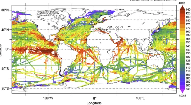
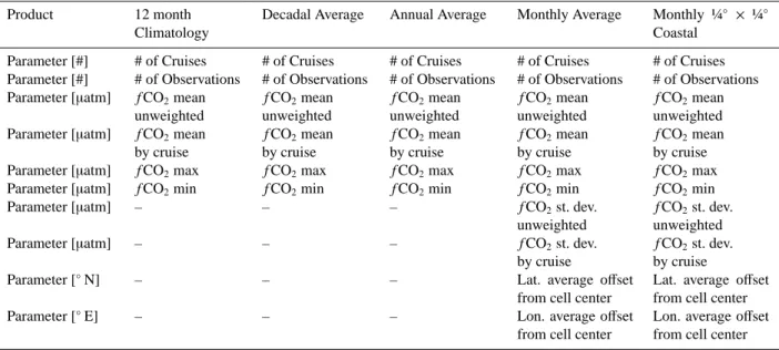
Surface Ocean CO2 Atlas (SOCAT) gridded data products

The Surface Ocean CO 2 Atlas (SOCAT) project was initiated by the international marine carbon science commu- nity in 2007 with the aim of providing a comprehensive, pub-

RNA-seq data obtained throughout our in vitro differentiation model of human B cells ( 7 ) support these results and show an UPR response well before cells are secreting

Clément Agret , Céline Gottin , Alexis Dereeper , Christine Tranchant-Dubreuil , Annie Chateau , Anne Dievart , Gautier Sarah , Alban Mancheron , Guilhem Sempéré , Manuel Ruiz

Of the 520 plumes from the five sources considered in both use cases respectively, only 295 for the Balkans and 203 or 194 for Norway (low and high release respectively) can be used

The following guidance is given in the GAMP: “Screening criteria should be determined nationally, and expressed in practical terms, either total effective dose (or total

(c-d) Relationship between delta soil organic carbon (SOC) (x-axis) with delta topographic wetness index as well as delta mean corrected crop water stress index (y-axis) for all the

The residence permit for private reasons based on humanitarian grounds (Status A of this report) allows for the Minister to grant an authorisation to stay in the country to

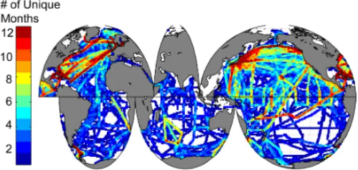
Regions for version 2 are the Coastal Seas, the North Atlantic, Tropical Atlantic, North Pacific, Tropical Pacific, Indian Ocean and Southern Oceans and a newly defined Arctic