A&A 591, A108 (2016) DOI:10.1051/0004-6361/201628196 c ESO 2016
Astronomy
&
Astrophysics
Azimuthal asymmetries in the debris disk around HD 61005
A massive collision of planetesimals?
?,??J. Olofsson
1, 2, 3, M. Samland
3, H. Avenhaus
4, 2, C. Caceres
1, 2, Th. Henning
3, A. Moór
5, J. Milli
6, H. Canovas
1, 2,
S. P. Quanz
7, M. R. Schreiber
1, 2, J.-C. Augereau
8, 9, A. Bayo
1, 2, A. Bazzon
7, J.-L. Beuzit
8, 9, A. Boccaletti
10,
E. Buenzli
7, S. Casassus
4, 2, G. Chauvin
8, 9, C. Dominik
11, S. Desidera
12, M. Feldt
3, R. Gratton
12, M. Janson
3, 13,
A.-M. Lagrange
8, 9, M. Langlois
14, 15, J. Lannier
8, 9, A.-L. Maire
12, 3, D. Mesa
12, C. Pinte
16, 8, D. Rouan
10, G. Salter
15,
C. Thalmann
7, and A. Vigan
15, 6(Affiliations can be found after the references) Received 26 January 2016/ Accepted 16 April 2016
ABSTRACT
Context.Debris disks offer valuable insights into the latest stages of circumstellar disk evolution, and can possibly help us to trace the outcomes of planetary formation processes. In the age range 10 to 100 Myr, most of the gas is expected to have been removed from the system, giant planets (if any) must have already been formed, and the formation of terrestrial planets may be on-going. Pluto-sized planetesimals, and their debris released in a collisional cascade, are under their mutual gravitational influence, which may result into non-axisymmetric structures in the debris disk.
Aims.High angular resolution observations are required to investigate these effects and constrain the dynamical evolution of debris disks.
Further-more, multi-wavelength observations can provide information about the dust dynamics by probing different grain sizes.
Methods.Here we present new VLT/SPHERE and ALMA observations of the debris disk around the 40 Myr-old solar-type star HD 61005. We
resolve the disk at unprecedented resolution both in the near-infrared (in scattered and polarized light) and at millimeter wavelengths. We perform a detailed modeling of these observations, including the spectral energy distribution.
Results.Thanks to the new observations, we propose a solution for both the radial and azimuthal distribution of the dust grains in the debris disk. We find that the disk has a moderate eccentricity (e ∼ 0.1) and that the dust density is two times larger at the pericenter compared to the apocenter.
Conclusions.With no giant planets detected in our observations, we investigate alternative explanations besides planet-disk interactions to interpret the inferred disk morphology. We postulate that the morphology of the disk could be the consequence of a massive collision between ∼1000 km-sized bodies at ∼61 au. If this interpretation holds, it would put stringent constraints on the formation of massive planetesimals at large distances from the star.
Key words. circumstellar matter – zodiacal dust – techniques: high angular resolution
1. Introduction
Debris disks are the leftovers of star and planetary formation processes (seeWyatt 2008;Krivov 2010;Matthews et al. 2014, for recent reviews). Departure from photospheric emission at infrared (IR) wavelengths was first discovered around Vega (Aumann et al. 1984) using the Infrared Astronomical Satellite (IRAS). This excess emission was originally thought to be the remnant of the cloud out of which Vega formed. Several decades later, we now know that the dusty “debris” responsible for the IR emission are arranged in a disk comparable to the Edgeworth-Kuiper belt in the solar system. The dust grains, with sizes between a few µm to a few millimeters, located at tens of au
? Based on observations made with ESO Telescopes at the
Paranal Observatory under programs ID 095.C-0298 and 095.C-0273. Based on Herschel observations, OBSIDs: 1342270977, 1342270978, 1342270979, 1342270989, and 1342255147. Herschel is an ESA space observatory with science instruments provided by European-led Princi-pal Investigator consortia and with important participation from NASA.
?? The reduced images as FITS files, and data of Fig. 1 are only
available at the CDS via anonymous ftp to
cdsarc.u-strasbg.fr(130.79.128.5) or via
http://cdsarc.u-strasbg.fr/viz-bin/qcat?J/A+A/591/A108
from the central star are heated by the stellar radiation and re-emit at mid-IR and mm wavelengths. Since the original discov-ery, and mostly thanks to space-based missions such as the In-frared Space Observatory, Spitzer, and Herschel, several hundred of main sequence stars are known to harbor debris disks (e.g., Eiroa et al. 2013;Chen et al. 2014).
Recent decades have seen incredible progress in the field of disk observations (e.g.,Augereau et al. 1999;Kalas et al. 2005; Buenzli et al. 2010;Lebreton et al. 2012;Millar-Blanchaer et al. 2015). Observations with ever improving spatial resolution have revealed asymmetric disks (e.g., Lagrange et al. 2016; Kalas et al. 2015) as well as complex, moving, small-scale struc-tures (Boccaletti et al. 2015). Nonetheless, spatially resolved observations of debris disks remain relatively rare and even though there are theoretical works focusing on the dynam-ical evolution of debris disks (e.g., Dominik & Decin 2003; Kenyon & Bromley 2006), they still need to be confronted with the observations. The current paradigm is that the primordial gas-rich proto-planetary disks are thought to have a half-life time of about 2−3 Myr (Hernández et al. 2007). As a disk evolves Pluto-sized planetesimals can form (Johansen et al. 2015) along with giant planets which may accrete their mass from the gas reservoir (core accretion or gravitational instability scenarios).
Table 1. Log for the VLT/SPHERE and ALMA observations.
VLT/SPHERE
Observing date Prog. ID Instrument Mode Filter Seeing Airmass Coherence time
[YYYY-MM-DD] [00] [ms]
2015-02-03 95.C-0298 IRDIFS H2H3/YJ 0.67 1.01 22.0
2015-03-30 95.C-0298 IRDIFS_EXT K1K2/YH 1.24 1.04 1.7
2015-05-01 95.C-0273 IRDIS DPI B_H 1.16 1.29 1.7
ALMA
Observing date Prog. ID Mode Resolution Frequency range PWV Integration
[YYYY-MM-DD] [kHz] [GHz] [mm] [s]
2014-03-20 2012.1.00437.S Continuum 31 250.00 211.91−228.97 0.79 120.96
Gas 488.28 230.05−230.99
After a few Myr, the gaseous content is quickly removed from the disk by efficient processes such as photo-evaporation (e.g., Alexander et al. 2006;Owen et al. 2011). Only already formed planets, planetesimals and dust grains will thus remain while the disk enters its debris disk phase. After a short phase of runaway growth, terrestrial planets may form in the inner gions of the disk, with Pluto-sized bodies in the outer re-gions, via chaotic growth of these oligarchs, on a timescale of 10−100 Myr (Kenyon & Bromley 2006, 2008, 2010). The time evolution of the entire system then becomes more regu-lar and less chaotic. The km-sized bodies, arranged in one or more planetesimal belt(s), evolve under their mutual gravita-tional influence. Through collisions, they continuously release small particles in a collisional cascade. Small dust grains, in turn, are removed from the system either by radiation pressure or Poynting-Robertson drag. Therefore, one can consider that after ∼100 Myr, planetary formation has stopped. The system is left with one (or more) planetesimal belt(s) and, quite possibly, with planets of various masses. By observing systems in the range 10−100 Myr, one can therefore study the time evolution of de-bris disks. Spatially resolved images can provide constraints on the radial and azimuthal distribution of the dust, giving us insight about the dynamics at stake in these systems.
Here, we present Very Large Telescope (VLT) Spectro-Polarimetric High-contrast Exoplanet REsearch (SPHERE) and Atacama Large Millimeter/submillimeter Array (ALMA) obser-vations of the debris disk around the solar type star HD 61005 (G8V), located at a distance of 35.4 ± 1.1 pc (van Leeuwen 2007). The age of the system is believed to be within 40+10−30Myr old, based on membership of the Argus association (Desidera et al. 2011; De Silva et al. 2013; Elliott et al. 2014). The uncertainties for the age are mostly related to the disper-sion in ages reported in the literature for both the Argus as-sociation and the IC 321 super cluster. In the last ten years, it has been spatially resolved on multiple occasions with sev-eral instruments; Hines et al. (2007, Hubble Space Telescope HST/NICMOS);Maness et al.(2009, HST/ACS);Buenzli et al. (2010, VLT/NaCo); Ricarte et al. (2013, Submillimeter Array SMA); andSchneider et al.(2014, HST/STIS). The disk earned its nickname of The Moth because of the swept-back wings first revealed in the HST observations of Hines et al. (2007). The wings may originate from the interaction between the interstellar medium (ISM) and the disk itself; as the star moves through the local ISM, (small) dust grains are set on eccentric orbits, drifting away from the central star.
WhileHines et al. (2007) andManess et al. (2009) mostly studied the wings, the study presented inBuenzli et al. (2010)
resolved the debris disk as a ring, thanks to the better angular res-olution provided by the NaCo instrument. They found the disk to be almost edge-on (i= 84.3 ± 1◦), to have a semi-major axis of
61.25 ± 0.85 au with an eccentricity of e= 0.045 ± 0.015, which translates into an offset of 2.75 ± 0.85 au of the star with respect to the disk. A brightness asymmetry between the two ansae is observed, which cannot be fully explained by the off-centering. No planets were detected byBuenzli et al.(2010), for observa-tions that should, in principle, have detected planets with masses starting from a few Jupiter masses. The integrated luminosity of the disk is large at IR wavelengths (Ldisk/L? ∼ 3 × 10⁻³) and
is best modeled by two spatially separated dust belts. The main dust belt is the one located at ∼60 au presented inBuenzli et al. (2010), but a warm component is usually required to reproduce the spectral energy distribution (SED).Ricarte et al.(2013) ar-gue that this additional belt is mandatory to match the SED at about 20 µm, however its location remains unconstrained. In this paper, we focus on constraining the properties of the debris disk which is resolved at unprecedented angular resolution at both near-IR and mm wavelengths. Studying the properties and ori-gin of the swept-back wings is beyond the scope of this paper, since they are marginally detected with these observations.
2. Observations, data processing, and stellar parameters
Table1summarizes the VLT/SPHERE and ALMA observations presented in this study.
2.1. VLT/SPHERE IRDIS observations and data reduction The star HD 61005 was observed with the VLT/SPHERE (Beuzit et al. 2008), within the guaranteed time consortium. The observations were obtained in different instrumental set-ups in February, March, and May 2015, using the dual-band imager (IRDIS,Dohlen et al. 2008;Vigan et al. 2010), the integral field spectrograph (IFS,Claudi et al. 2008), and the dual-polarization imager (IRDIS DPI,Langlois et al. 2014).
2.1.1. IRDIS dual-band observations
The February observations were conducted in the H2H3 dual
band (centered on 1.59 and 1.67 µm) for IRDIS and the Y J-band (0.95−1.35 µm, at spectral resolution R ∼ 54) for IFS. The March observations used the K1K2filters (centered on 2.11 and
2.25 µm) for IRDIS and the Y H-band (0.95−1.65 µm, R ∼ 33) for IFS. All of these observations were performed using an
apodized Lyot coronagraph, consisting of a focal mask with a di-ameter of 185 milli-arcsec (N_ALC_YJH_S) and a correspond-ing pupil mask. Coronagraphic observations were performed in pupil stabilized mode to use angular differential imaging (ADI) post-processing (Marois et al. 2006) to attenuate resid-ual speckle noise. The observation strategy can be summarized as follows: 1) photometric calibration: imaging of star offset from coronagraph mask to obtain PSF for relative photomet-ric calibration; 2) centering: imaging with star behind mask with four artificially induced satellite spots for centering; 3) sci-ence: coronagraphic sequence; 4) centering: same as point two; 5) photometric calibration: same as point one; 6) sky back-ground observation using same DIT as coronagraphic sequence. Finally, true north and plate scale are determined using astromet-ric calibrators as part of the SPHERE GTO survey for each run (Maire et al. 2016).
Basic reduction of the IRDIS data (background subtrac-tion, flat fielding, centering) was performed using the SPHERE Data Reduction Handling (DRH) pipeline (Pavlov et al. 2008, version 15.0). The output consists of cubes for each filter, re-centered onto a common origin using the satellite spot reference. The cubes are then corrected for the true north position de-termined from the astrometric calibrations and for distortion. We collapsed the two filters together to increase the signal-to-noise ratio (S/N), and from now on we will refer to the H2H3
and K1K2 datasets as H and K observations, respectively. The
datacubes in both bands were then processed using a prin-cipal component analysis (PCA, using the implementation of the scikit-learn Python package,Pedregosa et al. 2011) ap-proach from all frames within the data-cube.
2.1.2. IRDIS dual polarization observations
On May 1, 2015, the target was observed using IRDIS in DPI mode in H-band. The same coronagraph was used for these ob-servations. IRDIS DPI splits the light into two perpendicular po-larization directions imaged at the same time on the same detec-tor. Full cycles of half-wave plate (HWP) positions (0, 22.5, 45, and 67.5◦) were taken to construct the Stokes Q and U vectors.
The strategy of the observations was to take as long exposures as possible without saturating the detector just outside the corona-graph to achieve the best possible inner working angle as well as the best S/N for the outer part of the disk. Two integration times (DIT= 64 s with a total integration time of 768 s and DIT = 16 s with a total integration time of 3008 s) were used. IRDIS suffers from a de-polarization effect at certain detector position angles, which depend on the parallactic angle at the time of observation. Because the parallactic angle changed rapidly during the obser-vations, we updated the detector angle at regular intervals.
The DPI data were reduced using a custom pipeline that is different to the DRH pipeline, which closely follows the pro-cesses described in Avenhaus et al. (2014), using the double-difference method (see also Canovas et al. 2011) to construct Stokes Q and U vectors from the data. The pipeline has been adapted to suit the IRDIS instrument. The data were centered us-ing the centerus-ing frames taken just before and after the science observations. A de-rotation was applied to bring all files to the same orientation (see section above). Furthermore, the frames were corrected to take account of the fact that the IRDIS pixel scale differs slightly (∼0.6%) in the two principal detector direc-tions. The files were then corrected for true north as determined for IRDIS.
Because scattered light in an optically thin (debris) disk is ex-pected to be polarized perpendicular to the line between the star
and the image point in question, we then construct local Stokes Q and U vectors, denoted Qφand Uφ(see alsoBenisty et al. 2015). In case of single scattering of the stellar light, Qφ is expected to contain the disk signal, while Uφ is expected to contain no signal (with possible exceptions when the optical depth is large, Canovas et al. 2015) but noise on the same level as the Qφimage and can serve as a noise estimator. Qφ and Uφ can be
calcu-lated as:
Qφ= +Q cos(2Φ) + U sin(2Φ)
Uφ= −Q sin(2Φ) + U cos(2Φ), (1)
where φ refers to the azimuth in polar coordinates, andΦ is the position angle of the location of interest (x, y), with respect to the stellar location (x0, y0) as:
Φ = arctanx − x0
y − y0 + θ,
(2) where θ corrects for instrumental effects such as a small mis-alignment of the half-wave plate.
During the data reduction process, one HWP cycle equiva-lent to 256 s of data (DIT = 16 s) was taken out because the telescope had lost tracking for a short amount of time, rendering this data unusable. The result are two pairs of Qφand Uφimages, one for the DIT= 16 s and DIT = 64 s observations each. These were then combined with a weighted average to produce the final Qφand Uφimages.
2.1.3. IFS observations
The IFS data proved difficult to be properly reduced at the time of this analysis, mainly because of centering problems. Present-ing and analyzPresent-ing these observations will be postponed for a fu-ture study.
2.1.4. Processed images
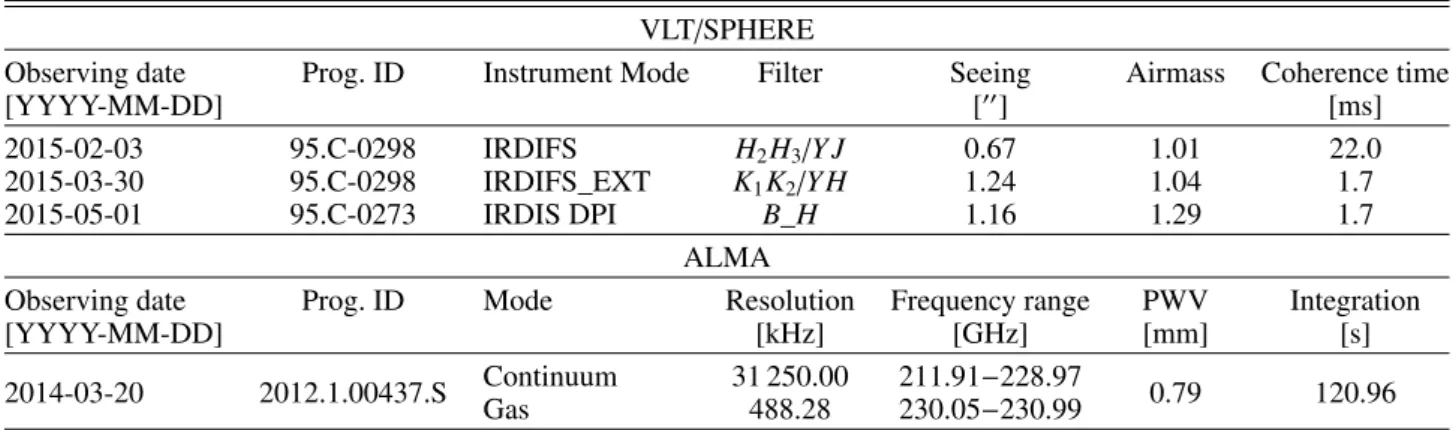
Figure1 shows the final reduction for our dataset (with a cen-tral mask of radius 0.1500). The top row displays the IRDIS ADI data in H and K-bands (left and middle panels, respectively), and the IRDIS DPI Qφ image (right), all with a linear stretch. For each image, the bottom row shows a S/N map, with a linear stretch between [−3σ, 3σ]. The noise map is calculated from the reduced images and represents the standard deviation in concen-tric annuli, centered on the star, with a constant width (2 pixels). We did not mask out the disk when computing the noise maps, hence the uncertainties might be slightly over-estimated. For the DPI observations, the noise map is computed from the Uφimage which does not seem to contain any signal from the disk (Fig.C.1 shows the Uφimage with the same linear stretch as the Qφimage in Fig.1).
We note that the disk is not homogeneously detected at high S/N. The east side is detected at larger S/N in all datasets and it appears brighter than the west side. Such asymmetry, already reported inBuenzli et al.(2010), are further investigated in this paper. For the sake of simplicity, in the rest of the paper, we refer to the ADI and DPI datasets as “scattered” and “polarized” observations, respectively. Strictly speaking, this is not correct as polarized photons must have been scattered by dust grains. 2.2. ALMA observations
HD 61005 was observed with ALMA in Band 6 (PI: David Rodriguez, program 2012.1.00437.S), in the frequency range
Fig. 1.Reduced SPHERE observations of HD 61005 used in the analysis. North is up, East is left. From left to right; IRDIS ADI in H and K-bands (PCA with 6 components), and IRDIS DPI Qφin H-band. Top row shows the data in linear stretch, with a central mask of 0.1500, and the bottom
rowshows estimated signal-to-noise maps (see text for detail), with a stretch between [−3σ, 3σ].
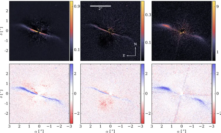
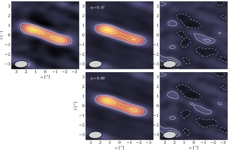
Fig. 2.From left to right: observations, best-fit model and residuals of the ALMA data. For all panels the color map is a linear stretch between −0.27 and 1.23 mJy/beam. The standard deviation estimated in an empty region of the observations is of 0.09 mJy/beam. For both the observations and the model the contours are set at [3, 5, 7.5, 10]σ, and [−σ, σ] for the residuals (no residuals beyond the 2σ level). The beam size is shown in the lower left corner of each panels.
211.97−230.99 GHz. The target was observed several times, with precipitable water vapor ranging from 5.19 to 0.79 mm. We only kept the observations performed on the 20 of March 2014 for which the water vapor was minimum. Out of the four spectral windows, three were used to derive the continuum emission (211.97−228.97 GHz, with a 31 250 kHz resolution), while the last one was used to search for CO gas emission (230.05−230.99 GHz, with a 488.28 kHz resolution), which was not detected. Data processing was performed within CASA us-ing the standard scripts provided by the observatory. We only
kept the spectral windows used for the continuum observations and averaged the complex visibilities along the 128 different spectral channels (while flagging points with negative weights). FigureC.2shows the (u, v) plane coverage for the continuum ob-servations, with minimum and maximum baselines of 11.8 and 334.9 m, respectively. The reconstructed image (with so-called briggs weighting and pixel size of 0.1300) is shown in the left
panel of Fig.2(sensitivity of 0.09 mJy/beam). The beam size is 1.3600× 0.7300 (48 au × 26 au) with a position angle of −86.5◦.
Table 2. Broadband photometric measurements of HD 61005, and the equivalent widths of the far-IR filters (see text for details).
λ Fν σ EW Instrument [µm] [mJy] [mJy] [µm] 0.428 895.17 14.02 TYCHO B 0.534 1810.23 18.34 TYCHO V 1.235 2753.74 65.94 2MASS J 1.662 2440.48 103.40 2MASS H 2.159 1738.75 38.43 2MASS Ks 3.353 819.28 31.69 WISE W1 4.603 453.05 8.76 WISE W2 11.56 78.40 1.08 WISE W3 22.09 44.28 1.55 WISE W4 68.92 717.00 5.33 21.41 PACS Blue 97.90 703.58 6.84 31.29 PACS Green 153.94 472.65 14.58 69.76 PACS Red 251.50 235.6 13.5 67.61 SPIRE PSW 352.83 118.9 7.6 95.75 SPIRE PMW 511.60 49.8 5.2 185.67 SPIRE PLW 1300.0a 4.6 0.7 105.40 ALMA Band 6
Notes.(a)Results from the modeling of the ALMA data (Sect.3).
from these observations, but we do estimate it when modeling the complex visibilities (Sect.3).
2.3. Spectral energy distribution
The star HD 61005 was observed by Herschel (Pilbratt et al. 2010) with the Photodetector Array Camera and Spectrometer instrument (PACS, Poglitsch et al. 2010), within the program OT2_tcurrie_1. The observation numbers (OBSID) are the two pairs 1342270977, 1342270978 and 1342270979, 1342270980 for the 70 µm and 100 µm observations, respectively. The 160 µm map used the four OBSID combined. The data were processed using the HIPE software (build 12.0.2083,Ott 2010), the very same way as described in Olofsson et al. (2013). HD 61005 was also observed with the Spectral and Photometric Imag-ing Receiver instrument (SPIRE, Griffin et al. 2010) in small scan map mode (OBSID: 1342255147 within the program OT2_kstape01_1). We used the Timeline Fitter task in HIPE to derive SPIRE photometry for our target. Calibration er-rors (∼5.5%, Bendo et al. 2013) are included in the uncertain-ties. We also gathered photometric observations using VOSA1 (Bayo et al. 2008) and the dataset used to build the SED can be found in Table2. The meaning of the third column is explained in Sect.5.
Finally, we downloaded the Spitzer/IRS spectrum from the Cornell Atlas of Spitzer/IRS Sources database2 (Lebouteiller et al.2011).
2.4. Stellar parameters
The stellar photospheric model is taken from the ATLAS9 Ku-rucz library (Castelli et al. 1997) with an effective temperature of T? = 5500 K (Casagrande et al. 2011). With the dilution factor used to scale the photospheric model to the optical and near-IR
1 http://svo2.cab.inta-csic.es/theory/vosa/
2 The Cornell Atlas of Spitzer/IRS Sources is a product of the Infrared
Science Center at Cornell University, supported by NASA and JPL.
http://cassis.sirtf.com/atlas/query.shtml
photometric measurements, at a distance of 35.4 pc, we find a ra-dius R?= 0.84 R . We derived a luminosity of L?= 0.58 L . To
derive the stellar mass, which will become important when dis-cussing the dust properties and the effect of radiation pressure on dust grains, we use isochrones from Siess et al.(2000), for an age of 40 Myr and effective temperature of 5500 K. We find that the stellar mass must be of about 1.1 M (the
cor-responding luminosity matching our estimated L?). We find a slightly smaller mass (1 M ) when using the isochrones from
Baraffe et al. (2015), but the differences may arise from differ-ent model prescriptions (e.g. overshooting). In the following, we adopt a mass of 1.1 M . The SED with the broadband
photo-metric measurements, the Spitzer/IRS spectrum as well as the photospheric model are shown in Fig.7of Sect.5.
2.5. Preamble on the modeling strategy
In this study, we aim to model observations from different fa-cilities, at different wavelengths, using different techniques (in-terferometry and direct imaging). Therefore, before detailing the modeling strategy for each individual dataset, we provide a quick preamble on the methodology.
We first model the ALMA data (Sect.3) assuming a circu-lar disk, fitting the reference radius (r0, where the dust density
peaks), the outer slope for the dust density distribution (αout),
the position angle (φ), the inclination (i), and the total flux at 1.3 mm ( f1300).
Prior to the modeling of the SPHERE observations, we at-tempt to constrain some of the dust properties, to limit the num-ber of free parameters. We use the best fit results for the inclina-tion and posiinclina-tion angle from the modeling of the ALMA data to derive the polarized intensity as a function of the azimuthal angle from the Qφ image. We constrain the minimum and maximum grain sizes (smin and smax, respectively) as well as the porosity
fraction of the dust grains (Sect.4.1). This enables us to reduce the pool of free parameters when modeling the SPHERE DPI observations. For the SPHERE ADI observations, we use the Henyey-Greenstein approximation for the phase function, which disconnects the modeling process from the aforementioned dust properties. Thanks to the great complementarity between the ADI and DPI observations, we model them simultaneously to best constrain the azimuthal and radial dust density distribution (Sect.4).
Finally, in Sect.5, we model the SED of HD 61005, using the results inferred from the modeling of the SPHERE data on the location of the disk to derive stringent constraints on the dust properties (minimum grain size, dust composition, and total dust mass).
3. The parent planetesimal belt: constraints from the ALMA observations
Roughly speaking, different wavelengths trace different grain sizes. Therefore, we chose to model the ALMA observations in-dependently of the SPHERE ones, the latter probing the small dust grains in the debris disk while the millimeter observations most likely trace a population of larger grains that more closely follow the parent planetesimals’ belt.
3.1. Modeling strategy
The modeling of the ALMA observations is performed in the Fourier space, attempting to reproduce both the real and
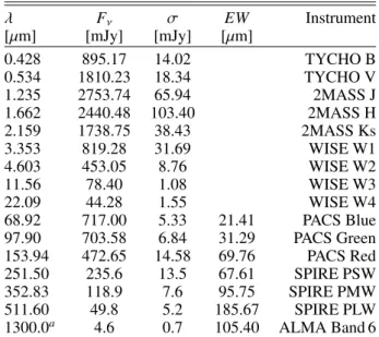
Fig. 3.One- and two-dimensional (diagonal and lower triangle, respec-tively) projections of the posterior probability distributions for the re-sults of the modeling of the ALMA observations.
imaginary parts of the complex visibilities (averaged along the spectral dimension). In AppendixA, we explain how we gen-erate synthetic images and the different notations are summa-rized in TableC.1. From a synthetic image at the wavelength of 1.3 mm, we first scale the total flux of the image to the free pa-rameter f1300 (in mJy) before computing the Fourier transform
of the image. We then interpolate the Fourier transform at the spatial frequencies of the observations. The goodness of fit is the sum of the weights (estimated in CASA3) times the squared dif-ference between the observed and modeled complex visibilities (the weights are proportional to 1/σ2). We consider the follow-ing free parameters: the inclination i, the position angle φ, the to-tal flux of the disk at 1.3 mm f1300, the reference radius4r0, and
the outer power-law slope for the dust distribution αout, which is
parametrized as n ∝ r r0 !−2αin + r r0 !−2αout −1/2 , (3)
where r is the distance from the star and n the number density. The inner power-law slope is set to αin = 5, preliminary tests
indicating this parameter is poorly constrained by the observa-tions. To find the most probable solution, we use an affine invari-ant ensemble sampler Monte-Carlo Markov Chain, implemented in the emcee package, using 200 walkers, a burn-in phase of 500 iterations and a total length of the chains of 2000 iterations after the burn-in phase. At the end of the run, we find that the mean acceptance fraction (the mean fraction of steps accepted for each walker within the chain) is of 0.48 (a good sign of con-vergence and stability, Gelman & Rubin 1992). The maximum auto-correlation time for all the parameters is of 60 steps, indi-cating that the chains should have stabilized by the end of the simulations.
3 The absolute values of the weights derived within CASA may be
inaccurate but their relative values are not.
4 Here we assume the disk is circular.
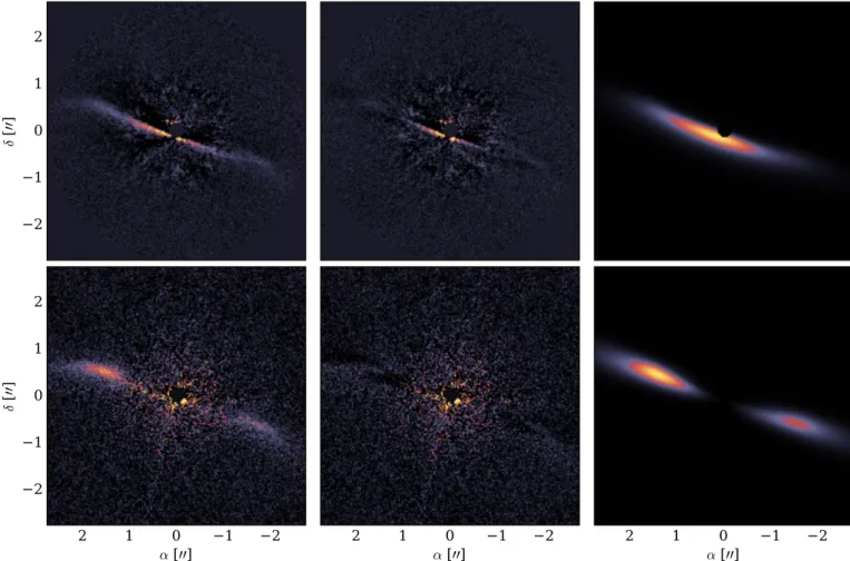
Table 3. Best fit results for the modeling of the ALMA observations.
Parameter Uniform prior σkde Best-fit value
r0[au] [40, 80] 0.2 66.4+6.1−8.7 αout [−15, −1.5] 0.1 −6.6+1.4−6.1 φ [◦] [55, 85] 0.1 70.7+1.9 −2.3 i[◦] [79, 89] 0.1 84.5+2.9−2.5 f1300[mJy] [1, 20] 0.1 4.6+0.7−0.6 3.2. Results
The projected posterior probability distributions are displayed in Fig.3, for the different free parameters (using the triangle Python package, Foreman-Mackey et al. 2014). To derive the best-fit values as well as the uncertainties, we smooth the dis-tributions with a kernel density estimator (the width of the Gaussian kernel σkde are reported in Table3), and the best-fit
value is the peak position of the distribution. The confidence in-tervals (a1, a2) for the parameter a are estimated as follows:
Z a1 amin p(a)da= Z amax a2 p(a)da=1 − γ 2 , (4)
where γ = 0.68 and p(a) is the smoothed posterior probabil-ity distribution (integral normalized to 1) for parameter a (e.g., Pinte et al. 2008). We note that not all the distributions reach zero on each side of their maximum (especially for αout and
i) and, therefore, these uncertainties should be treated care-fully. Table3 summarizes our results for the modeling of the Band 6 observations, and Fig.2shows the observations, the best-fit model, and the residuals (from left to right). The synthetic im-age of the best fit model is processed through CASA (using the ft method with the same antenna configuration as the observa-tions) and the image is reconstructed with the clean algorithm with the same parameters as for the observations. We note that there are some residuals on the east side that may suggest that the disk is brighter on one side, even at mm wavelength. However, these residuals are below 3σ, therefore we cannot conclude they are significant. The apparent brightness asymmetry could be due to the asymmetric (u, v) coverage of the observations.
Overall, we find that most of the parameters are well con-strained, except for the outer power-law slope of the dust density distribution, for which we can safely exclude slopes shallower than αout = −4. This is explained by the beam size of the
ob-servations which is larger than the debris disk for steep values of αout. Otherwise, we find the reference radius of the disk to
be r0 ∼ 66 au, the position angle φ ∼ 70.7◦, the inclination
i ∼ 84.5◦, and the flux at 1.3 mm f
1300 ∼ 4.6 mJy. These
re-sults agree well with the parameters reported inBuenzli et al. (2010, i = 84.3 ± 1◦, φ = 70.3 ± 1◦, r0 = 61.25 ± 0.85 au) and
Ricarte et al.(2013, r0= 67±2 au, φ = 71.5±5◦). The relatively
large beam size of the ALMA observations can explain the slight discrepancy for r0 between the modeling of the ALMA data
and the value inferred byBuenzli et al. (2010). This value will be revisited when modeling the SPHERE observations (Sect.4). Ricarte et al. (2013) obtained a total flux of 7.2 ± 0.3 mJy at 1.3 mm with their SMA observations (Steele et al. 2016obtained 8.0 ± 0.8 mJy analyzing the same observations), while we find the total flux to be well constrained at 4.6 ± 0.7 mJy (within the SMA and ALMA respective 3σ uncertainties). The shortest baselines being of Bmin∼ 11 and 16 m (for the ALMA and SMA
are sensitive to are of the order of 14.200and 10.100, respectively (0.6λ/Bmin), much bigger than the disk. It is therefore unlikely
that flux from the disk is filtered out by the interferometers. The differences between the SMA and ALMA data may arise from missing frequencies, differences in beam sizes, or calibration un-certainties (the uncertaintites reported bySteele et al. 2016being more conservative than the ones reported byRicarte et al. 2013). Finally, we note that the famous wings responsible for the disk’s nickname are not detected in the ALMA data. Despite a good angular resolution, a disk model (without wings) can suc-cessfully reproduce the observations, and we see no trace of the wings in the residuals (with an rms of ∼0.09 mJy/beam). Our re-sults therefore agree with the ones ofRicarte et al.(2013); only small dust grains are likely present in the wings.
4. Constraining the dust radial distribution from the SPHERE observations
We model the SPHERE images by producing synthetic images at the central wavelength of the H-band observations, λc =
1.63 µm. Given the low S/N of the K-band ADI observations, preliminary attempts to model these data showed that the dust distribution cannot be better constrained than with the H-band observations. We therefore focus the modeling effort on the H-band ADI and DPI data.
Figure1highlights the complementarity of both the scattered and polarized light images; the ADI and DPI data have very dif-ferent S/N at the ansae and along the semi-minor axis of the disk. Combining both datasets, therefore, offers the opportunity to study the dust distribution in great detail.
The modeling process has a high dimensionality with many possible free parameters, and regions of intermediate to low S/N. Therefore, to obtain novel yet reliable constraints on the dust dis-tribution we choose to perform a prior analysis on the observa-tions to reduce the number of free parameters. Having a proper description of the polarized phase function prior to the modeling of the DPI observations greatly helps reducing the dimensional-ity of the modeling (e.g., the minimum and maximum grain sizes as well as the porosity of the dust grains). In this section, we first describe how the polarized phase function is derived and mod-eled, then we present the modeling strategy and summarize the results we obtain.
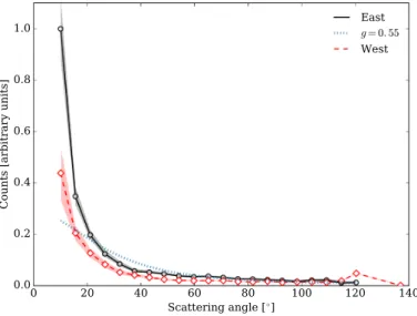
4.1. Phase function of the polarized light
To compute the polarized phase function from the DPI dataset, we define an elliptical mask with the following parameters: in-ner and outer radii (rinand rout), the inclination i, and the position
angle φ. For each pixel within the elliptical mask, we compute the scattering angle as the dot product of the line of sight and the location of the pixel with respect to the star. We divide the ellipti-cal mask in two, for the east and west sides and, for each side, we compute the minimum and maximum scattering angles. We then divide each side of the mask into 30 smaller regions correspond-ing to different bins of the phase function (see Fig.C.3for an il-lustration). Each pixel is multiplied by its squared distance to the star, to account for illumination effect. The measured phase func-tion is found by averaging the flux in the observafunc-tions, in each individual region. Since the observed uncertainties σiare not the
same for each pixel within a given intersection, the “average”
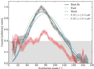
Fig. 4.Azimuthal dependency of the polarized intensity in the DPI H-band observations, in black and red for the East and West sides, re-spectively. The shaded curves are representative of the uncertainties es-timated from the noise map and the shaded gray area denotes low S/N regions estimated from the S/N map in Fig.1. The thin solid lines dis-play examples for different grain sizes for the same dust composition as the best fit.
uncertainty in the intersection is computed as follows: σ = N X i=1 1 σ2 i −1/2 , (5)
where N is the number of pixels in the considered region. The phase function is then normalized to its maximum value (east and west sides are divided by the same value).
For the elliptical mask, we use the best-fit results of the mod-eling of the ALMA observations (see Table3) for i and φ and choose rin and rout small and large enough (50 and 72 au,
re-spectively) so that they encompass the trace of the debris disk. Figure4 shows the phase function for the DPI H-band obser-vations, the east side being in black, and the west side in red. The uncertainties are shown in a shaded color, and the gray area indicates regions of low S/N, which were estimated from the S/N map derived from the Uφdata. As can be seen in Fig.1 (bot-tom right panel), the disk is only detected for a narrow range of azimuthal angles on the west side. This strongly suggests that we underestimated the uncertainties calculated using Eq. (5).
The difference in brightness between the two sides of the disk is striking in Fig.4and the east side appears almost twice as bright as the west side for most of the scattering angles. Even though the S/N for the west side is relatively low it seems that the polarized phase function peaks at an angle compatible with the east side.
To alleviate the number of free parameters, we aim to con-strain the grain size distribution for the modeling of the DPI ob-servations directly from the phase function displayed in Fig.4. We emphasise that we do not have access to the polarization de-gree (√(Q2+U2)/I) as we do not have an unbiased measure of the
total intensity I prior to the modeling. Indeed, the ADI process introduces self-subtraction effects (e.g.,Milli et al. 2012), which can eventually be quantified with a model that describes the ob-servations well (which we do not yet have). Since the west side suffers from low S/N, we perform the modeling on the east side’s phase function. To reproduce the phase function, we assume that the signal in the Qφimage is proportional to the size dependent
S12(s) element of the Müller matrix. The matrix enables us to
compute the Stokes vectors I and Q for the scattered and polar-ized light, respectively. Assuming single scattering event (rea-sonable assumption in low density environment such as debris disks), the scattered light will be the product of the first diagonal element of the matrix S11 times the stellar intensity I0. The
po-larized intensity will be proportional to the second element of the first column of the matrix S12times I0. We compute S12for
dif-ferent grain sizes between sminand smax, using the Mie theory,
and we average S12 over a grain size distribution with a slope
p< 0 (dn(s) ∝ spds) as follows, Savg12 = Rsmax smin S12(s) × s pds Rsmax smin s pds · (6)
We then compute the best scaling factor fS12 (to be multiplied to
Savg12 ) that will minimize the difference between the profiles Savg12 and Sobs 12 (with uncertainties σ) fS12 = P Sobs 12 × S avg 12 σ2 P Savg12 σ 2 · (7)
We perform a simple grid search over the following parame-ters: smin, smax, and the optical properties of the dust grains. We
fix p = −3.5, as expected for a collisional cascade in a debris disk (Dohnanyi 1969). For the dust composition, we consider a base medium of amorphous silicate with olivine stoichiometry (MgFeSiO4,Dorschner et al. 1995) to which we can add some
porosity using the Bruggeman mixing rule. The minimum grain size can vary between 0.01 and 10 µm. To constrain the max-imum grain size, we vary the quantity ∆s (=smax− smin)
be-tween 0.01 and 100 µm (in log space), and finally the porosity can change by steps of 10%. We find that the polarized phase function at 1.63 µm is best reproduced by small spherical dust grains, with typical sizes in the range 0.3 ≤ s ≤ 0.35 µm and a porosity fraction of ∼80%. The best-fit solution is shown with a thick cyan line in Fig.4, and reproduces well both the overall shape and the peak position of the observed phase function. Also shown in Fig.4are two examples for different grain size distri-butions around 0.25−0.3 µm and 0.35−0.4 µm, to illustrate how sensitive the phase function is with respect to the grain sizes. We note that, within such a narrow range of sizes, the value of the slope p of the grain size distribution remains unconstrained. In this section, we assumed that the polarized flux is directly pro-portional to S12, while it is also related to the dust density in the
disk. In the rest of this paper, we try to determine the azimuthal distribution of the dust in the disk. Therefore, this prior analysis must be regarded as a first order approximation. The motivation of this prior analysis was to reduce the dimensionality of the modeling, but it also comes at a slight cost in the interpretation of the grain size distribution. The main conclusion of this section is that it does not seem that we observed large dust grains (which would have a stronger S12 signal at small scattering angles). In
Sect.6.1we discuss this result further, but it could also be the consequence of low S/N along the semi-minor axis of the disk. 4.2. Modeling strategy
Since both the ADI and DPI datasets were taken at the same wavelength, for a given set of parameters we compute
two images: an unpolarized light image using the Henyey-Greenstein (HG) analytical prescription of phase function S11
(Henyey & Greenstein 1941) and a polarized light image us-ing the Mie theory. Usus-ing the HG approximation, which is parametrized by the anisotropic scattering factor g (−1 ≤ g ≤ 1), gives us more control when trying to reproduce the observed phase function (hence less free parameters to be considered dur-ing the modeldur-ing). To reproduce the DPI observations, we use the grain properties derived previously (Sect.4.1). The absorp-tion and scattering efficiencies, as well as the Müller matrix ele-ment S12, are computed with the Mie theory, which is valid for
compact spherical grains. This approach may not appear self-consistent, but it is a way to disentangle the modeling of unpo-larized and pounpo-larized light that may not be well accounted for by spherical grains (e.g.,Milli et al. 2015).
The pool of free parameters includes the reference radius r0,
the inclination i, the position angle φ, the opening angle ψ, and the outer power-law slope αout for the dust density distribution.
Preliminary tests indicated that we can hardly constrain the inner power-law slope, so we fixed αin= 5. This enables us to focus on
other parameters that describe the geometry of the debris disk. For instance,Buenzli et al.(2010) conclude that the eccentricity of the disk was not enough to explain the brightness asymmetry between the east and the west sides, and we aim to address this interpretation of previous observations. Therefore, we include the eccentricity e, the rotation angleΦe, the density damping η,
and its azimuthal shape (via the width w of the Gaussian profile) and its reference angleΦη(see AppendixA). The azimuthal
pro-file has the shape of a Gaussian propro-file with a σ= w, a peak of 1 for the azimuthal angleΦηand a minimum value of η ≥ 0 (hence
an amplitude of 1 − η).
Because we now consider azimuthal variations for the dust density distribution, it is parametrized slightly differently. The semi-major axis of the disk is defined as r0/(1 − e2). Although
the formal denomination of r0is the so-called semi latus rectum,
we will simply refer to it as the reference radius in the rest of the analysis. The radius at which the dust density peaks now depends on the azimuthal angle θ. This radius rθis defined as r0/(1 + e ×
cosθ), and the azimuth-dependent dust density distribution n(θ) is parametrized similarly to Eq. (3), replacing r0with rθfor each
azimuthal angle.
The dust mass Mdust is not varied, but the synthetic images
are scaled during the fitting process. For the polarized images, the modeled image is the absolute value of the Stokes Qφ
param-eter (we are assuming that there are no multiple scattering events in the debris disk). We scale the modeled image by a factor fDPI,
which is found analytically to minimize the residuals (similarly to Eq. (7)). For the ADI dataset, this approach is not possible because the post-processing of the data cube can introduce self-subtraction effects. We therefore opted for a forward modeling strategy, similar to the one described inThalmann et al.(2014). For a given set of parameters, we compute one synthetic image at the wavelength 1.63 µm. We then produce a cube of 64 images, each one rotated to match the parallactic angles of each frame of the observations (total rotation of 93.3◦). Each frame of the cube
of synthetic images is multiplied by fADIand is then subtracted
from the corresponding observed frame. The PCA process is performed, keeping only the six main components. Another ap-proach would be to perform the PCA on the observations, save the coefficients, and apply them to the modeled cube. But the ob-servations contain signal from the disk that may be accounted for in some of the principal components (even though they should be similarly subtracted in the modeled cube). Therefore, to ensure as little subtraction as possible, we chose to perform the PCA on
Table 4. Best fit results for the ADI and DPI H-band observations.
Parameter Uniform prior σkde Best-fit value
r0[au] [40, 80] 0.1 60.4+0.8−0.5 i[◦] [75, 88] 0.1 84.1+0.2 −0.2 αout [−10, −1.75] 0.01 −2.70+0.1−0.1 e [0, 0.6] 0.0025 0.093+0.018−0.014 Φe[◦] [0, 360] 1. 127.3+12.7−4.3 φ [◦] [65, 75] 0.1 70.6+0.2 −0.3 η [0, 1] 0.0025 0.47+0.02−0.04 Φη[◦] [0, 360] 1.0 138.1+7.2−5.6 w [◦] [5, 180] 1.0 51.7+8.8 −3.2 ψ [0.02, 0.12] 0.005 0.058+0.001−0.002 g [0, 0.95] 0.001 0.54+0.01−0.02 fADI [3, 8.5] 0.01 6.20+0.09−0.07
the model-subtracted cube. The end goal being to minimize the flux in the final image.
The goodness of the fit is the sum of the squared ratio be-tween the final images (residuals for the scattered and polarized data) and the noise map (bottom row of Fig.1). For the mod-eling of both the ADI and DPI observations, we therefore have a total of 12 free parameters: r0, i, αout, e, Φe, φ, η, Φη, w, ψ,
g, and fADI. Here, we also use the emcee Python package, with
100 so-called walkers in the chain, and first burn in 500 runs for each of these walkers. We then run the chain for 2000 iterations in total (seeMillar-Blanchaer et al. 2015for a similar modeling approach). To speed up the process, we cropped and re-sampled the SPHERE images. The size of one pixel in the new image (or cube) is resampled to be 2.25 times bigger than in the original images, the size of the new image being 200 × 200 pixels, and we use a central mask of radius 0.1500. We chose not to convolve the synthetic images by a PSF because the cropped and down-sampled images have a pixel size of 0.02800, while the
approx-imation of the instrumental PSF with a Gaussian profile would have a width of 0.02400 (approximating the PSF as an Airy disk
for an 8 m telescope). At the end of the run, we find that the mean acceptance fraction (the mean fraction of steps accepted for each walker within the chain) is of 0.35, with a maximum auto-correlation time of 79 steps.
4.3. Results
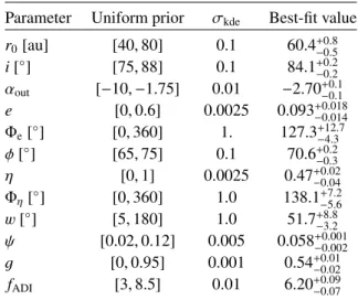
The projected posterior probability distributions are displayed in Fig.B.1, for the different free parameters. To derive the best-fit values as well as the uncertainties, we proceed similarly as in Sect.3.2. The results are presented in Table4and Fig.5shows the observations, the residuals and the best-fit models (from left to right) for the ADI and the DPI data (top and bottom rows, respectively).
All parameters seem to be well constrained. The most prob-able solution has a semi-major axis of 60.9 au (r0/[1−e2]) for
an eccentricity of 0.093. With a rotation angle of Φe ∼ 127◦
the pericenter is located slightly toward the observer, on the east side5. An azimuthal density variation seems to be necessary to
5 ForΦ
e = 180◦, the pericenter would be along the semi-major axis
on the east side. Smaller angles would move the pericenter towards the observer, while larger angles would move the pericenter towards the back side of the disk.
reproduce the observations with a damping factor η of ∼0.47 with a reference angle of ∼138◦ (hence almost co-located with
the pericenter of the eccentric disk). The azimuthal variation of the dust density distribution is a Gaussian profile with a width of ∼50◦. The position angle and inclination are
consis-tent with the results fromBuenzli et al.(2010). The aspect ratio of ψ ∼ h/r ∼ 0.06 agrees well with numerical simulations of the vertical structures of debris disks (e.g.,Thebault 2009). Finally, the phase function is anisotropic for low scattering angles with g ∼ 0.54. The dust density distribution for the best-fit model, viewed from above the disk, is displayed in Fig.B.2.
Nonetheless, as shown in the residuals of the ADI observa-tions, our best-fit model does not manage to remove all the sig-nal along the semi-minor axis of the disk. It successfully sup-presses most of the signal at larger scattering angles, but the best-fit model seems to fail at properly describing the scatter-ing at smaller angles. We tried to implement a phase function with two weighted HG functions, but could not significantly im-prove the residuals. We included all the “basic” parameters re-lated to the geometry of the disk (i, φ, r0, ψ) and yet failed to
perfectly match the observations. Possible explanations can be related to the phase function (the HG phase function remains an approximation), the radial segregation of the grain size dis-tribution, or the azimuthal dust density distribution (this will be further discussed in Sect.6.1). We crudely assumed a Gaussian profile for the azimuthal distribution, but the actual distribution could be skewed in one or another direction which could explain the brighter region along the semi-minor axis. Another (highly speculative but interesting) explanation could be that we may be seeing an inner disk. Because of the high inclination of the disk, an inner dust belt may appear to the observer as if it was merging with the main belt. The main challenge with this explanation is that we see no indication of this type of a belt in the DPI obser-vations, but the noise is larger in the innermost regions of this dataset. One possible way to address this point would be to de-tect gas, which could trace velocities compatible with a radius smaller than 61 au. Yet no CO was detected in the ALMA obser-vations (Sect.6.2).
5. Constraining the dust mineralogy from the SED The SED of the debris disk around HD 61005 is constructed from the fluxes reported in Table2and the Spitzer/IRS spectrum. Modeling an SED from unresolved observations is a degenerate problem. We are basically trying to find the adequate tempera-ture of the grains, which can be changed either by their radial dis-tances, their sizes, or their nature. The modeling of the SPHERE images provide strong constraints on the geometric parameters of the disk, and we can therefore focus on better constraining the dust properties.
5.1. Modeling the thermal emission from the disk
To model the SED of HD 61005, for a given set of parameters, the goodness of fit is computed as
χ2=X i ωi× " Fobs(λi) − F?(λi) − Fmodel(λi) σi #2 , (8)
where Fobsis the observed flux with its associated uncertainty
σi, F? the stellar contribution, and Fmodel the modeled thermal
emission of the debris disk. The ωivalues are weights to the
Fig. 5.Left to right: observed, residuals, and best-fit models for the ADI and DPI datasets (top and bottom, respectively).
to account for the fact that we simultaneously model broad-band photometric observations (e.g., Herschel/PACS) and spec-troscopic observations (Spitzer/IRS): two adjacent points in the IRS spectrum do not have the same significance as PACS 70 and 100 µm observations. We therefore opt for a similar strat-egy to the one described in Ballering et al. (2013). We pute the average spectral resolution of the IRS data and com-pare it to the equivalent widths of the broadband filters. One IRS point will have a weight ω = 1 and broadband photomet-ric point will have a weight equal to the number of IRS points that would fit in the corresponding equivalent width of the fil-ter. In Table2, we report the equivalent widths for the various instruments used to model the thermal emission in the far-IR. These values were taken from the Spanish Virtual Observatory filter profile service6. For the ALMA Band 6 observations, we assumed the equivalent width to be equal to the spectral range (105 µm).
To account for different mineralogical components, we use amorphous silicate grains of olivine stoichiometry (MgFeSiO4,
Dorschner et al. 1995, ρ = 3.5 g cm−3) and amorphous water ices (Li & Greenberg 1998, ρ= 1.2 g cm−3). To mimic porosity,
we also add the fraction of vacuum to the pool of free param-eters. We mix the optical constants of the different dust com-ponents, using the Bruggeman mixing theory, and the Mie the-ory to compute the absorption coefficients Qabs. Since computing
Qabsfor large grain sizes can be the bottle-neck when computing
thousands of models, we first created a library of opacity files (smin = 0.01 µm and smax = 5 mm, with steps of 10% for the
6 http://svo2.cab.inta-csic.es/theory/fps3/
water ices, and porosity fractions). During the modeling process, the appropriate Qabs are drawn and interpolated for the proper
grain size distribution and composition.
The free parameters include the grain size distribution (smin
and p, we fix smax = 5 mm), the relative fractions for the
frac-tions of amorphous water ices and porosity, and the inner and outer slopes for the dust density (αinand αout, respectively). We
fix the reference radius r0 to the best-fit results of the
model-ing of the SPHERE observations. For each set of parameters the dust mass Mdust is found by scaling the thermal emission of the
model to the observed SED (similarly to Eq. (7)). The values for the dust mass are saved for posterior estimation of their corre-sponding uncertainties. To speed up the modeling of the SED, we neglect the non-azimuthal dust density distribution derived from the analysis of the SPHERE data and assume the disk to be a circular ring. We use the emcee package to search for the most probable model, using 100 walkers, burning the first 500 runs for each walker, and then running the chain for 1000 more iter-ations. The acceptance fraction at the end of the run is of 0.28 (and a maximum auto-correlation time across all parameters of 72 steps).
5.2. Results
Table5 summarizes the best fit results and the derived un-certainties and projected posterior probability distributions for each parameter are displayed in Fig.6. The SED of HD 61005, along with the photometric and spectroscopic observations, the photospheric model, and the best-fit model are shown in Fig.7. The shape of the mid- to far-IR excess is well reproduced by
Fig. 6.Posterior probability distributions for the modeling of the SED. The solid lines indicate the most probable value, and the vertical dashed lines indicate the derived uncertainties.
Fig. 7.Spectral energy distribution of HD 61005. Photometric measure-ments are shown in red, along with the Spitzer/IRS spectrum (uncer-tainties, shown in gray, are 3σ, most of them being smaller than the symbol). The dashed gray line is the photospheric model, the black and cyan lines are the best fit models (including the stellar contribution, but with and without the inner component, see text for details).
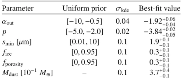
Table 5. Best-fit results for the modeling of the SED.
Parameter Uniform prior σkde Best-fit value
αout [−10, −0.5] 0.04 −1.92+0.06−0.04 p [−5.0, −2.0] 0.02 −3.84+0.02−0.05 smin[µm] [0.01, 10] 0.1 1.9+0.1−0.1 fice [0, 0.95] 0.1 0.3+0.1−0.1 fporosity [0, 0.95] 0.1 0.3+0.1−0.1 Mdust[10−1M⊕] – 0.1 3.7+0.4−0.1
our model, but the turn-off point, where the excess emission starts, is not well matched (near λ ∼ 20 µm). This hints towards the presence of an additional component, an inner disk that has also been postulated by many authors in the literature (e.g., Morales et al. 2011; Ballering et al. 2013; Ricarte et al. 2013; Chen et al. 2014). Even when using detailed dust properties (in-stead of Planck functions at single temperatures) to model the excess, the best-fit model still underestimates the flux in the mid-IR beyond 3σ. To constrain the properties of an additional belt, we fit a Planck function to the residuals (the only free parame-ter being the temperature, the scaling to the residuals being done similarly to Eq. (7)). We find the temperature of the Planck func-tion to best reproduce the residuals to be ∼220 K. In Fig.7, the
Planckfunction is shown as a dotted-dashed black line and the final best-fit model (stellar contribution plus the inner and outer belts) as the solid black line. To assess the relevance of adding the inner disk we follow a similar approach as in Moór et al. (2015b, and references therein) and use the Akaike Information Criterion (AIC). We find that the addition of the inner compo-nent significantly improves the final model (the AIC including the inner belt is about 80% of the AIC without it), and therefore is deemed necessary to reproduce the whole SED of the disk around HD 61005.
Our modeling results suggest that the outer slope of the dust density distribution is relatively shallow, which would indicate that most of the grains responsible for the emission are located in an extended disk. The minimum grain size is found to be ∼1.9 µm, and the grain size distribution has a steep slope of p ∼ −3.84. The composition of the grains would be a mixture of amorphous silicate grains with small fraction of water ices and porosity. The total dust mass (between smin and smax) is of
the order of 0.37 M⊕.
6. Discussion
In the following, we try to put together the results of the mod-eling of the ALMA, SPHERE datasets as well as of the SED. We discuss what can be inferred regarding the dust properties, the gas content, the morphology of the disk to better charac-terize what is happening in this system. Because we modeled several datasets (ALMA, SPHERE, SED), Table6summarizes which parameters are constrained with which datasets, to clarify the discussion.
6.1. Dust properties
6.1.1. Self-subtraction corrected phase function
With a satisfying model for the scattered light, we can further investigate the phase function in the SPHERE ADI H-band ob-servations. Indeed, the model enables us to estimate the self-subtraction introduced by the PCA analysis. To do so, we first perform the PCA on the raw data cube and save the resulting co-efficients. We then take the best-fit model, produce a data cube at the proper parallactic angles, project it into the new orthog-onal basis found for the observations, and multiply this projec-tion with the same coefficients as for the raw observations (e.g., Soummer et al. 2012). This provides us with an estimate of the signal from the disk that is subtracted when doing the PCA. The attenuation is estimated by the ratio rcorr between this estimate
and the original model. When deriving the phase function for the ADI dataset (similarly to Sect.4.1), each pixel is multiplied by the quantity 1/(1 − rcorr). Figure8shows the phase function
Table 6. Summary of the modeling strategy adopted in this study.
Parameter ALMA data Polarized intensity SPHERE DPI SPHERE ADI SED
[1] [2] [3] [4] [5]
r0[au] Fitted – Fitted Fitted Fixed to [3,4]
αin 5 – 5 5 5
αout Fitted – Fitted Fitted Fitted
φ [◦] Fitted Fixed to [1] Fitted Fitted –
i[◦] Fitted Fixed to [1] Fitted Fitted –
f1300[mJy] Fitted – – – –
smin 0.1 µm Fitted Fixed to [2] – Fitted
smax 5 mm Fitted Fixed to [2] – 5 mm
fporosity 0 Fitted Fixed to [2] – Fitted
e 0 – Fitted Fitted – Φe[◦] – – Fitted Fitted – η 1 – Fitted Fitted – Φη[◦] – – Fitted Fitted – w [◦] – – Fitted Fitted – ψ 0.05 – Fitted Fitted – g – – – Fitted – fADI – – – Fitted – p −3.5 −3.5 −3.5 −3.5 Fitted fice 0 0 – – Fitted Mdust[M⊕] – – – – Fitted
Notes. Even though the SPHERE DPI and ADI data are fitted simultaneously, we separated the entries to better see dependencies. A dash denotes that the parameter is irrelevant during the fitting of a given dataset.
Fig. 8.Phase function derived from the ADI H-band observations, cor-rected for self-subtraction effects (see text for details).
derived for the east and west sides (black and red, respectively). The bump at ∼120◦ on the west side is an artifact introduced by rcorr(low signal in the disk model leads to an erroneous
cor-rection factor). In Fig.8, we also show the phase function de-rived during the modeling (for g = 0.55), scaled to the phase function of the east for scattering angles larger than 40◦. The in-ferred HG function appears to be a relatively good representation of the corrected phase function for scattering angles larger than ∼50◦, but severely fails to reproduce it at smaller angles. This
would be an explanation for the strong residuals along the semi-minor axis in Fig.5. Overall, this suggests quite extreme forward scattering in the disk around HD 61005 – a result that remains model-dependent since the PCA attenuation is estimated from our results (see also Milli et al. 2016, for a similar discussion
for the disk around HR 4796 A). Nonetheless, the strong peak of scattering for small angles (down to ∼10◦) strongly points
to-wards the presence of large dust grains in the debris disk. How-ever, this seems in contradiction with the prior analysis of the DPI dataset where we had to actually reject the presence of large dust grains (s ∼ 0.3 µm). For the SED, we need a whole range of sizes (from µm- to mm-sized grains), but the emission is actually dominated by the smaller grains (discussed further in this section). Numerous studies of debris disks around different stars (e.g.,Rodigas et al. 2015;Lebreton et al. 2012;Milli et al. 2015,2016) already reported and discussed similar issues in rec-onciling the modeling results of different kind of observations. Throughout this paper, for their computational merits, we have either used the Mie theory or the HG prescription while both of them may not be accurate descriptions of the nature of the dust grains.
6.1.2. Reconciling different observations
To try to reconcile the different dust properties inferred from our modeling results, the radial extent of the disk is interesting to discuss. The ALMA observations point towards a narrow belt (αout ≤ −5), while the SED, ADI, and DPI observations
sug-gest that the disk is extended (αout ∼ −2 or −3). To assess the
typical grain sizes we probe with the SED, we computed the integrated infrared luminosity for each grain size bins between sminand smax, and built the cumulative distribution function. We
find that more than 98% of the disk infrared luminosity is ac-counted for by dust grains smaller than 5 µm. The rest of the (very steep) grain size distribution contributes marginally to the total emission. This means that for the DPI observations and the SED, we are observing an extended disk containing small dust grains. We computed the β ratio between the radiation pres-sure and gravitational forces as in Burns et al. (1979), assum-ing L∗ = 0.58 L and M∗ = 1.1 M . For the dust composition
sblow ∼ 0.8 µm, for which β ≤ 0.5, should remain on bound
or-bits (assuming they were released on circular oror-bits). There is a small discrepancy between sblowand the minimum grain size we
found (smin ∼ 2 µm) but as discussed inPawellek et al.(2014),
this could be caused by the assumption of spherical grains when modeling the SED. Assuming our inferred dust composition is not too far off compared to the real composition of the dust grains, it seems that radiation pressure should be efficient for (sub-) µm-sized grains. Consequently, the parent belt (inferred from the ALMA data) would be fairly narrow, but small grains placed on eccentric orbits (or even unbound) owing to radi-ation pressure make the disk look more extended at near-IR wavelengths.
The strong forward scattering peak derived from the cor-rected phase function from the ADI observations suggests the presence of large grains in an extended disk, which seems in con-tradiction with the aforementioned scenario. Nonetheless, ac-cording toMin et al.(2016), large dust aggregates behave like large grains (the size of the whole aggregate) in scattered light and like small grains (the size of the individual monomers) for polarized light. Such aggregates also display mild backward scattering that we do not detect with our observations but may be the consequence of low S/N along the back side of the disk.
Therefore, we hypothesize that the parent planetesimals are arranged in a narrow belt (traced by ALMA) and that the small-size end of the grain small-size distribution consists of dust aggregates that are pushed away by radiation pressure. This makes the disk appear extended in the SPHERE observations and when mod-eling the SED. For future studies of this system, it would be interesting to implement a radial segregation of the grain size distribution (varying dn(s) as a function of r, see for instance Stark et al. 2014for a discussion of the phase function depend-ing on the radial distance).
6.2. Gas mass upper limits
No CO emission was detected in the ALMA data, and we follow a similar procedure to that ofMatrà et al.(2015) andMoór et al. (2015a) to derive upper limits for the CO gas mass. We extract the spectrum from the datacube reduced within CASA, centered around 230.5 GHz (12CO 2−1). The upper limit for the CO mass
was determined as MCO= 4πmd2? hν2−1A2−1 S2−1 x2−1 , (9)
where m is the mass of the CO molecule, d? the distance of
the star, ν2−1 the frequency of the transition, A2−1 the Einstein
coefficient7, x
2−1 the fractional population of the upper level,
and S2−1 the observed integrated line flux. The fractional level
was calculated assuming local thermal equilibrium, using the Boltzmann equation, with a temperature of 20 K (as discussed inMoór et al. 2015a, MCOis not strongly dependent on the
tem-perature). S2−1was computed from the spectrum as Srms∆v
√ N, where∆v is the channel velocity width, N the number of chan-nels over a width of 15 km s−1(centered at the local standard of
rest velocity, vLSR), and Srmsthe standard deviation of the
spec-trum within that velocity range. From the heliocentric radial ve-locity of 22.5 km s−1(Desidera et al. 2011), we obtain a vLSR of
3.68 km s−1. Assuming optically thin gas, this leads to an upper
limit of 6.9 × 10⁻⁷M⊕. As discussed inMatrà et al.(2015), the
LTE hypothesis may not hold in low-density environment and
7 Taken from the SPLATALOGUE catalog athttp://www.cv.nrao.
edu/php/splat/
our upper limit could underestimate the CO gas mass. In the ISM the CO/H2abundance is 10−4and with our inferred dust mass of
∼0.37 M⊕ (for our grain size distribution), this would lead to a
gas-to-dust ratio that is much smaller than unity. However, it is unlikely that this ratio will remain the same in a circumstellar disk because of effects such as photo-dissociation. Overall, with the available observations leading to a non-detection, and given the several assumptions made (LTE, CO/H2ratio) we can hardly
conclude on the gas-to-dust ratio on the debris disk. This ques-tion should be addressed by future, deeper CO observaques-tions (or other species than the CO molecule).
6.3. Stirring of the planetesimals
In the last few years, theoretical works have aimed at characteriz-ing the time evolution of debris disks (e.g.,Kenyon & Bromley 2006,2008). One of the purpose of these studies has been to better understand the growth of planetesimals to sizes of about a thousand km, in the framework of terrestrial planetary forma-tion. It is believed that once these large bodies have been formed, they stir the population of smaller planetesimals. The stirring increases the relative velocities of these planetesimals and in-creases their chances of collisions, therefore initiating a colli-sional cascade. According to these models, collisions between planetesimals become destructive only once a Pluto-sized object is formed. Since the timescale for the growth of planetesimals scales with the distance r to the star, self-stirring is thought to be an inside-out process. Here, we follow a similar approach to that described in Moór et al. (2015b), who studied several de-bris disks spatially resolved with the Herschel observatory. They examined if the disks in their sample are consistent with a self-stirring scenario. To achieve this, they compared the timescale for forming a 1000 km-sized object in a self-stirred debris disk with the age of the stars. To quantify this timescale t1000(in Myr),
we used Eq. (41) fromKenyon & Bromley(2008), which we re-call below:
t1000= 145x−1.15m (r/80) 3(2M
/M?)3/2[Myr], (10)
where r is the distance of the dust belt, and xm is a scaling
fac-tor to parametrize the disk’s initial surface density (the higher, the more massive).Mustill & Wyatt(2009) argue that xmvalues
larger than 10 are highly unlikely since the initial disk would have been gravitationally unstable. Assuming that the timescale for the growth of the planetesimals is the age of the system (i.e., t1000 = 40 Myr), we find that xmshould be of the order of about
3.3 (for r = 61 au). This value would suggest that either the primordial disk was ∼3 times more massive than the minimum-mass solar nebula, or that other sources of stirring (e.g., induced by a planet) need to be taken into consideration for this system. Debris disks with known planets, such as the ones studied in Moór et al.(2015b, e.g., HR 8799, β Pictoris, HD 95086), have much larger xmvalues (≥10), while most of the debris disks
usu-ally have values for xmsmaller than 3. It is therefore reasonable
to assume that the disk around HD 61005 is bright because self-stirring by planetesimals has recently started. It does not imply that alternative stirring mechanisms should not be considered, but based on the distance of the dust belt and the age of the system, it is not mandatory to invoke the presence of a massive planet to explain what is currently observed.
6.4. An eccentric and asymmetric disk
With the new SPHERE observations, we confirm the findings of Buenzli et al. (2010) that the disk displays a strong brightness
Fig. 9.From left to right: observations, models including some of the results of the SPHERE modeling, and residuals. Top row is for η= 0.47 and the bottom row for η= 0.6. For all panels the color map is a linear stretch between −0.27 and 1.23 mJy/beam. For both the observations and the model the contours are set at [3, 5, 7.5, 10]σ, and [−2, −1, 1, 2]σ for the residuals. The beam size is shown in the lower left corner of each panels.
asymmetry. Both the ADI and DPI observations show that the eastern side is brighter than the western side at an unprecedented angular resolution. The asymmetry is detected both in scattered light along the semi-minor axis (ADI dataset) and in scattered and polarized light along the semi-major axis (NACO observa-tions ofBuenzli et al. 2010and DPI observations, respectively). When modeling the observations, we had to include a density damping factor along the azimuthal direction to reproduce the SPHERE observations. From preliminary tests, the DPI dataset (in which the brightness asymmetry is most visible) cannot be properly reproduced without these azimuthal variations. There-fore, we argue it can hardly be a scattering artifact and that it is, indeed, most likely related to a dust density enhancement in the disk.
On the other hand, the ALMA observations do not display such a strong asymmetry at first glance. To further investigate if the best fit model to the SPHERE observations is compatible with the ALMA data, we generated models including eccentric-ity and azimuthal variations. We took the best fit model to the ALMA data (Table3), and the following additional parameters from Table4: e = 0.093, Φe = 127◦, w = 52◦,Φη = 138◦,
and two values for η (0.47 and 0.6). Figure9shows the compar-ison between these models and the observations. For η = 0.47 (derived from the SPHERE observations), the brightness of the western side is slightly underestimated but the residuals barely reach the 2σ level. For η= 0.6, the model becomes more similar to the observations and the residuals do not reach the 2σ level. Consequently, we cannot exclude that the disk shows departure
from centro-symmetry in the ALMA data, but the sensitivity of the observations does not allow us to put meaningful constraints on the azimuthal variations for the population of large grains. We can exclude damping factors of η ∼ 0.5 to the 2σ level, but a value of 0.6 cannot be ruled out based on the available observations.
6.4.1. Possible planet-disk interactions?
Massive planets are often invoked to explain the eccentricity of a debris disk since the planet may shepherd it. The case of Fomalhaut is a good example of these types of studies. The disk shows an eccentricity comparable to the one of HD 61005 (e ∼ 0.11 ± 0.1, Kalas et al. 2005) and a candidate compan-ion was detected byKalas et al.(2008). Studies such as the one of Beust et al.(2014) investigate in detail the possible interac-tions between the planet and the planetesimal in the disk. In the last two decades, many numerical works have been led to in-vestigate how planets can shape debris disks (e.g.,Wyatt et al. 1999; Wyatt 2006; Nesvold et al. 2013; Pearce & Wyatt 2014; Faramaz et al. 2014), or how the planetesimals evolve within their mutual gravitational interactions (e.g., Kral et al. 2015; Jackson et al. 2014).
Via secular interactions, an eccentric planet can shape the de-bris disk. Because of differential precession, the planet-disk in-teractions can result in a (short-lived) spiral arm (Mouillet et al. 1997; Wyatt 2005). Then, when taking into account the ef-fect of collisions in the disk, the spiral quickly dissipates