January 9, 2010
Transiting exoplanets from the CoRoT space mission
IX. CoRoT-6b: a transiting ’hot Jupiter’ planet in an 8.9d orbit around a
low-metallicity star
?M. Fridlund
1, G. H´ebrard
2, R. Alonso
3,15, M. Deleuil
3, D. Gandolfi
10, M. Gillon
15,19, H. Bruntt
5, A. Alapini
6, Sz.
Csizmadia
11, T. Guillot
16, H. Lammer
13, S. Aigrain
6,24, J.M. Almenara
9,23, M. Auvergne
5, A. Baglin
5, P. Barge
3, P.
Bord´e
4, F. Bouchy
2,22, J. Cabrera
11, L. Carone
12, S. Carpano
1, H. J. Deeg
9,23, R. De la Reza
17, R. Dvorak
18, A.
Erikson
11, S. Ferraz-Mello
20, E. Guenther
10,9, P. Gondoin
1, R. den Hartog
1,7, A. Hatzes
10, L. Jorda
3, A. L´eger
4, A.
Llebaria
3, P. Magain
19, T. Mazeh
8, C. Moutou
3, M. Ollivier
4, M. P¨atzold
12, D. Queloz
15, H. Rauer
11,21, D. Rouan
3, B.
Samuel
4, J. Schneider
14, A. Shporer
8, B. Stecklum
10, B. Tingley
9,23, J. Weingrill
13, and G. Wuchterl
10 (Affiliations can be found after the references)Received 30 Nov 2009; accepted 4 Jan 2010
ABSTRACT
The CoRoT satellite exoplanetary team announces its sixth transiting planet in this paper. We describe and discuss the satellite observations as well as the complementary ground-based observations – photometric and spectroscopic – carried out to assess the planetary nature of the object and determine its specific physical parameters. The discovery reported here is a ‘hot Jupiter’ planet in an 8.9d orbit, 18 stellar radii, or 0.08 AU, away from its primary star, which is a solar-type star (F9V) with an estimated age of 3.0 Gyr. The planet mass is close to 3 times that of Jupiter. The star has a metallicity of 0.2 dex lower than the Sun, and a relatively high7Li abundance. While the light curve indicates a much higher level
of activity than, e.g., the Sun, there is no sign of activity spectroscopically in e.g., the [Ca ii] H&K lines.
Key words.techniques: photometric, spectroscopic, radial velocities – stars: planetary systems –
1. Introduction
Transits provide insights – currently impossible to gain with other techniques – into many aspects of the physics of extraso-lar planets (exoplanets) and are thus an extremely valuable tool. In spite of significant progress having been made in the detec-tion of transiting exoplanets from the ground, e.g., Super WASP (Christian et al. 2009), the method remains significantly ham-pered by observations through the atmosphere and most signifi-cantly by the interruptions caused by having an orbiting rotating Earth as an observing platform. This leads to the method being most sensitive to short orbital periods (of a few days).
The spacecraft CoRoT (Convection, Rotation, and planetary Transits) was successfully launched into a near-perfect orbit on 27 December 2006. This instrument was designed to discover and study in detail exoplanets for which the transits are difficult or impossible to detect from the ground. This concerns specifi-cally small planets or ‘Super-Earths’ (L´eger et al. 2009; Queloz et al. 2009), i.e., planets orbiting more active stars, e.g., CoRoT-2b, (Alonso et al. 2008) and with longer periods, e.g., CoRoT-4b, (Aigrain et al. 2008; Moutou et al. 2008). It is relatively easy for CoRoT to detect larger planets, similar in size to Jupiter, and a number of these have also been reported (Barge et al. 2008; Deleuil et al. 2008; Rauer et al. 2009). A second objective of the spacecraft is to study different aspects of micro-variability in stars, e.g., so-called p-modes in solar-type stars (Baglin et al.
?
The CoRoT space mission, launched on December 27, 2006, has been developed and is being operated by CNES, with the contribution of Austria, Belgium, Brazil, ESA, The Research and Scientific Support Department of ESA, Germany and Spain.
2006). In this paper, we concern ourselves exclusively with the former scientific goal – transiting exoplanets – and report the discovery of the ‘hot Jupiter’ object CoRoT-6b.
CoRoT observes from above the atmosphere, remaining pointed towards the same objects for up to longer than 150d with interruptions to the light curve equalling lower than 5% (Boisnard & Auvergne 2006). It is therefore capable of de-tecting transiting planets with periods in excess of 50d. With the launch of CoRoT, which provides essentially uninterrupted and long time sequences, the detection of small planets with radii only a few times the radius of the Earth has become possible (L´eger et al. 2009; Queloz et al. 2009). For exoplanets, the vi-sual magnitude range observable by CoRoT is about 11 - 16.5 and the photometric precision is close to the photon noise in the upper half of this range (Auvergne et al. 2009). Nevertheless, the identification of transit events is generally difficult being a demanding and complex process, which includes an ambitious follow-up program using ground-based observations (Deeg et al. 2009).
CoRoT-6b is the sixth secure transiting planet detected by CoRoT. This planet is one of only a handful of transiting planets with moderately long orbital periods (currently only 5 of a total of 62 such planets have periods longer than 5 days). In this pa-per, we present the photometric light curve of the star, as well as the photometric and spectroscopic ground-based follow-up ob-servations that establish the planetary nature of the object. We analyse the data and derive the physical properties of both the planet and its host star.
Fig. 1. The processed and normalised white light curve of the CoRoT-6 observation and the transits of the planet. It displays the total 144 days of data. The black (fuzzy) curve is the oversampled (32s) light curve, while the overlaid (blue, sharp) curve has been re-binned to a time-sampling of 1 hour. The ordinate in the plots is HJD - 2451545, corresponding to the HJD of the first of january of 2000 (the “CoRoT date” used as a zero-point for all light curves and ephemerises). This figure clearly demonstrate the high activity of CoRoT-6.
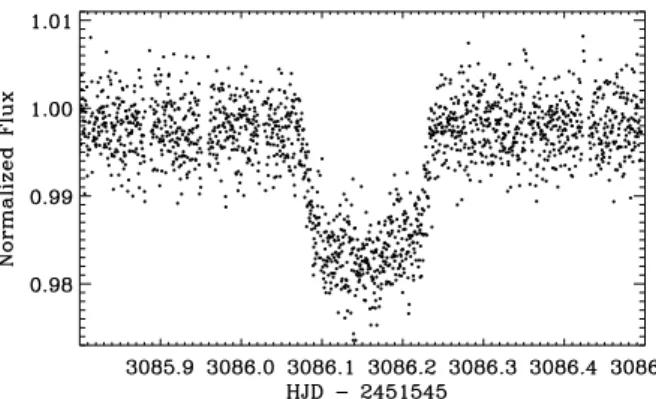
Fig. 2. Magnified portion of the processed and normalised light curve of CoRoT-6 displaying one of the transits.
2. Satellite observations and data processing
2.1. Light curve analysis
CoRoT-6b was discovered during the third ‘long’ observing run of CoRoT (second long observing run towards the Galactic cen-tre direction), which took place between April 15 and September 7, 2008. This field, which is designated LRc02, has centre coor-dinates of approximately α = 18h40mand δ = +6 deg . The
planet was detected transiting the CoRoT target 0106017681 (Deleuil et al. 2009), which is an mV = 13.9 star (see Table
1). CoRoT-6b was first noticed in the so-called ‘alarm-mode’, (Surace et al. 2008; Quentin et al. 2006), i.e., a first look at roughly processed data while a particular observing run is on-going and relatively little data is available. The first function of this ‘alarm mode’ is to change the time-sampling for a specific target from once every 512s to once every 32s. The second (very important) function is to alert and initiate the follow-up cam-paign already during the ongoing CoRoT observations. Because of the Earth’s orbital motion during a long pointing, sources ob-served during a run of 150 days or more, will disappear into the daytime sky very soon after the end of the CoRoT observing run. By waiting until the end of a long run, plus the time it takes to process the full data stream, the necessary follow-up
obser-vations would be delayed 5-6 months before the particular field re-emerges from behind the Sun.
The ephemeris of the midpoints of the eclipses was found to be
Tc= 2 454 595.6144±0.0002+ E?× (8.886593 ± 0.000004), (1)
where E?is the ordered number of the transit in question. After the detection of CoRoT-6b, the follow-up process was initiated early and the planetary nature of the object transit-ing CoRoT-6 was established very soon through ground-based spectroscopic observations (see below). The data presented in the current paper, however, contains the complete CoRoT light curve of the target, reduced using the latest version of the CoRoT calibration pipeline (June 2009). This latest version (ver-sion 2.1) of the pipeline includes:
– the correction for the CCD zero offset and gain;
– a correction for the background (as measured on the sky); – a correction for orbital effects;
– an improved spacecraft jitter correction.
The correction for the orbital effects consist of corrections for both the offset and background variations, an adjustment for pointing errors including effects on the spacecraft caused by the ingress/egress of the Earth’s shadow, cross talk in the electron-ics, and exposure time variations. Variations in the CCD tem-peratures are not corrected for but these effects are very small (Auvergne et al. 2009).
According to imagery and photometry of target fields ob-tained with the INT/WFC before the satellite observation and stored in the Exo-dat database (Deleuil et al. 2009), we esti-mate that flux contamination from the background stars falling inside the CoRoT-6’s photometric mask (Auvergne et al. 2009) is 2.8±0.7% of the total flux. Assuming that these contaminants are photometrically stable during the whole observing run, we sub-tract 2.8% of the median flux from the light curve. The estimated error in this contamination factor is taken into account during the bootstrap analysis described below.
The light curve from CoRoT for CoRoT-6 covers 144 days and comprises 331 397 samples, obtained with a ≥ 95 % duty cycle. In the case of the CoRoT target 0106017681, because
of its relative brightness, it was selected for both fast integra-tion (32s) and multi-color data taking from the beginning. For a number of targets, including CoRoT-6, the photometric mask is divided into three sections (‘red’, ‘green’ and ‘blue’) and thus three light curves are obtained. To obtain a higher S/N, these are added together for detection purposes, whereas the colors are used mainly to exclude contaminating objects and the ef-fect of stellar activity. In addition, the pipeline flags so-called ‘outliers’, i.e., sudden deviations from the light curve in one in-tegration bin. These are mostly caused by particle hits and most frequently during the satellite’s passage of the South Atlantic Anomaly, where even the shielding of the focal plane is not suf-ficient. The outliers are simply removed from the data stream before interpretation. Long-term effects caused by particle hits leaving remnant effects on the CCD detector with timescales of seconds, minutes, and even days (see Auvergne et al. (2009)) are left in the data stream by the pipeline and treated ‘manually’ in the subsequent analysis. The different timescales of the disconti-nuities that are observed of course have different frequencies. Significantly long timescale excursions are much rarer events and in the present case of CoRoT-6, as can be seen by Figs. 1 & 2, are virtually non-existent. After removal of transients, the resulting light curve has a duty cycle of ∼ 92%.
2.2. Transit parameters
We display the final light curve in Figs. 1 and 2, where we show both the complete data set covering the whole integration pe-riod as well as an enlarged portion of a section, around just one transit, which enhances the details. The final light curve shows some interesting characteristics. We first note that CoRoT-6b is an active star as are most of the other transiting planet host stars discovered by CoRoT (e.g., CoRoT-2b, -4b & -7b) . We detect a total of 15 transits with a maximum depth of ∼1.4%. The transits are clearly visible in the CoRoT light curve, as can be seen from the enlarged light curve in Fig. 2. We used three different fil-ter/model combinations to analyse the data. Initially, we used the same scheme as in some of the previous CoRoT planets (Barge et al. 2008; Alonso et al. 2008) and we refer to this scheme as the ‘Gimenez model’, but later included several alternative analyses for comparison and completion.
2.2.1. Polynomial fit filter and Gimenez model with Amoeba-algorithm
To extract the planetary and stellar parameters from the light curve, we use the same methodology as in Alonso et al. (2008). We recall here the main steps of the method: from the series of 15 transits, the orbital period and the transit epoch are determined by the trapezoidal fitting of the transit centres. The light curve is phase-folded to the ephemeris after performing a local linear fit to the region surrounding the transit centre to account for any local variations. The resulting light curve is displayed in Fig. 5 and has been binned in phase by 1.5 × 10⁻⁴in units of fraction of the orbital period. The error for each individual bin is calcu-lated as the dispersion in the data points inside the bin, divided by the square root of the number of points per bin. The physical parameters of the star and planet are then determined through χ2
analysis according to the method of Gim´enez (2006). We model the light curve with 6 free parameters (the transit centre (Tc), the
orbital phase at first contact (θ1), the radius ratio Rp/R?(k), the
orbital inclination i, and the u+and u−coefficients related to the
quadratic limb-darkening coefficients uaand ubthrough u+= ua
+ ub and u−= ua- ub(Gim´enez (2006) and references therein).
The transit fitting is then carried out with the same method as de-scribed in detail in Barge et al. (2008) and Alonso et al. (2008), using a bootstrap analysis to fully constrain the parameter space. The results are found in Table 2. For a detailed description of the limb darkening issue, we refer the reader to the discussion reported in Deleuil et al. (2008).
As mentioned above, we detected 15 transits during the com-plete run . After the light curve processing, the star displayed a transit signature with a period of 8.89 days (see Table 2) and a to-tal transit duration of 4.08±0.02 h. The phase-folded transit light curve, displayed in Fig. 5, exhibits a 1 σ rms noise of 4.58 ×10⁻⁴
(458 ppm). The time sampling here is ∼13s. The results of the analysis of the final light, combined with stellar parameters de-rived from spectra, allow us to determine the planetary parame-ters. As can be seen in Sect. 3.4, stellar modeling and light curve analysis provide consistent results for the stellar mass. The light curve then implies a planetary radius of Rp= 1.166±0.035 RJup.
2.2.2. Savitzky-Golay filter and Mandel & Agol model with Harmony Search algorithm
Independent filtering and fits were also carried out. The first is as follows. Here the light curve is processed in a different, more naive way than in the ‘Gimenez model’ (Sect. 2.2.1). After dividing the light curve by its median, a new curve was con-structed by convolving the resulting light curve with a fourth-order, 4096 × 4096 points Savitzky-Golay filter. The standard deviation of the differences between the measured and the con-volved light curves is then calculated. A 5σ clip is applied and the whole process is repeated until we do not find any more out-liers (spurious deviations from the mean > 5σ). A low-order (5) median-filter is then applied to increase the signal-to-noise ratio. To minimize the effect of the stellar activity, we fit the vicinity of every transit with a low order (2-3) polynomial excluding the transit points after which we divide the data with the resulting polynomial. After these steps, we fold the light curve and a bin-average is applied forming 2000 bins.
We used the Mandel & Agol (2002) model to perform the fit to the final, phase-folded light curve. We assumed a circular orbit and a 2.8% contaminant factor. Our five parameters were: the a/R?, k = Rpl/R? ratios, the inclination and the two limb
darkening coefficients ua, ub(we apply again the quadratic limb
darkening law). To find the best fit, we utilized the Harmony Search algorithm(Geem et al. 2001), which belongs to a family of genetic search algorithms. The 1σ errors were estimated from the width of the parameter distribution to be between χ2minand χ2
min+ 1. The results are:
– a/R?= 17.68 ± 0.26 – Rpl/R?= 0.1131 ± 0.0013 – i= 89◦ ·19 ± 0◦·25 – u+= 0.78 ± 0.08 – u−= 0.28 ± 0.13
These results are in very good agreement with the previous run (‘Gimenez model’), as is clearly evident by comparing with Table 2. The agreement is within the 3σ error limits of both the planet-to-stellar radius ratio and the limb-darkening and within the 1σ error bars for all the other parameters).
2.2.3. Iterative reconstruction filter and Mandel & Agol model with Levenberg-Marquardt algorithm
In this model, we start with the same light curve as described in Sect. 2.1. To circumvent the issue of varying data weights asso-ciated with different time sampling, the oversampled section of the light curve was rebinned to 512 s sampling. Outliers were then identified and clipped out using a moving median filter (see Aigrain et al. 2009 for details). Finally, we also discarded two segments of the light curve, in the CoRoT date ranges before 3031 days, and from 3152 to 3153.54 days (see Fig. 1), corre-sponding to two discontinuities in the light curve. The result-ing time-series was then fed into the Iterative Reconstruction Filter (IRF). A full description of this filter is given in Alapini & Aigrain (2009), but we repeat the basic principles of the method here for completeness. The IRF treats the light curve Y(i) as Y(i) = F(i) ∗ A(i) + R(i), where A(i) represents the signal at the period of the planet, which is a multiplicative term applied to the intrinsic stellar flux F(i), and R(i) represents the obser-vational noise. A(i) is obtained by folding the light curve at the period of the transit and smoothing it using a smoothing length of 0.0006 in phase, and the original light curve is then divided with the result, which is then run through an iterative non-linear filter (Aigrain & Irwin 2004) using a smoothing length of 0.5 days to estimate the stellar signal F(i). This signal in turn is re-moved from the original light curve and the process is iterated until the difference in residuals from one iteration to the next re-mains below 10−8for 3 consecutive iterations, which occurs after 129 iterations in this case. The IRF reconstructs all signal at the period of the transit unavoidably including stellar variability at this timescale if the star is active. This is the case for CoRoT-6, thus a 2nd order polynomial function is fitted about the transit of the phase-folded IRF-filtered light curve and divided into it. The light curve with the stellar signal removed is then fitted using the formalism of Mandel & Agol (2002) using quadratic limb darkening to generate model transit light curves, and the IDL implementation MPFIT of the Levenberg-Marquardt fitting al-gorithm (Markwardt 2009) to find the best model fit to the transit light curve. The adjusted parameters are: the epoch of the centre of the first transit in the light curve T0, the planet-to-star radius ratio Rpl/R?, the system scale a/R?, and the planet orbital
incli-nation with respect to the plane of view. The eccentricity is fixed to zero and the limb darkening coefficients are fixed to the values in Table 2. The uncertainties in the best-fit parameters are evalu-ated by circularly permuting the residuals 100 times, reevaluat-ing the parameters each time, and takreevaluat-ing the standard deviation of the values obtained for each parameter as the uncertainty in the parameter. The planet parameters found for CoRoT-6b with the above method are
– T0= 2454595.61433 ± 0.00017 – Rpl/R?= 0.1157 ± 0.0006
– a/R?= 17.0 ± 0.3
– i= 88◦ ·6 ± 0◦·1.
These values are again consistent with those obtained with the other modelling schemes, although this method favours a slightly more grazing transit.
2.2.4. Rotational modulation
A rotational modulation with an amplitude of ∼2 - 3 % is clearly present in the light curve, demonstrating clear signs of magnetic activity on the stellar photosphere. Determining the rotational period from star spot modulation is always fraught with
diffi-culty without a proper model e.g., Bonomo et al. (2009) of the distribution of the spots on the surface and their appearance and disappearance. This is because the true evolution of star spots is poorly understood and we can imagine that, for instance, when-ever a new spot appears it does so at a greater longitude than the previous one, introducing a systematic effect into the determina-tion of the rotadetermina-tional period. Carrying out the required modeling is beyond the scope of the present paper and we accept that our analysis will only provide a first order approximation. We start our analysis by dividing the light curve into three roughly equal sections. From these sections, we determine rotational periods of 6.3±0.5, 6.6±0.5, and 6.4±0.4 days respectively. We do not see any signs of systematic effects at this level of precision and simple averaging leads us then to a rotational period of 6.4±0.5 days for this star, a value that is consistent with the value of v sin iderived from spectral analysis in Sect. 3.4 (6.9±0.9 days).
2.3. Secondary eclipse
Despite the relatively long period of this transiting planet, we at-tempted a search for its secondary eclipse. Longer period plan-ets carry a double penalty in this aspect: first, we observe fewer eclipses for a given observation interval, causing a lower S/N and secondly, the larger value of a leads to a lower value of the Rpl/a ratio.
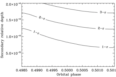
Using the same technique as Alonso et al. (2009), we calcu-lated the χ2fit using the same parameters as the observed tran-sit, at the time of the expected secondary eclipse. The result is presented in Fig. 6. We see no trace of a possible secondary oc-cultation. We derive a 3 σ upper limit of 1.8 × 10⁻⁴to the depth of the possible secondary transit in our data.
If the albedo of the planet was one, the expected depth of the secondary transit would be
Rpl
a !2
= 4.2 ± 0.2 × 10⁻⁵. (2)
Our data is thus not good enough in this case to show the sec-ondary light.
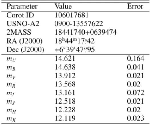
Table 1. Stellar parameters for CoRoT-6 with U, B, V, R, & I magnitudes from the Exo-dat database, and J, H and K magni-tudes mined from the 2MASS catalogue.
Parameter Value Error Corot ID 106017681 USNO-A2 0900-13557622 2MASS 18441740+0639474 RA (J2000) 18h44m17s ·42 Dec (J2000) +6◦ 390 4700 ·95 mU 14.621 0.164 mB 14.638 0.041 mV 13.912 0.021 mR 13.568 0.02 mI 13.161 0.072 mJ 12.518 0.021 mH 12.228 0.02 mK 12.119 0.023
3. Ground based follow-up observations
The CoRoT telescope has a large point spread function (PSF) and thus frequently background objects are found to
‘contami-Table 2. Parameters for CoRoT-6 and CoRoT-6b as derived from our analyses.
Parameter Value Uncertainty Unit Period 8.886593 0.000004 day Epoch (T0) 2 454 595.6144 0.0002 BJD θ1 0.00958 4.82057 × 10⁻⁵ k= Rp/R? 0.1169 0.0009 i 89.07 0.30 degrees u+ 0.586 0.068 u− -0.12 0.13 M1/3? / R? 0.993 0.018 a/R? 17.94 0.33 b(R?) 0.291 0.091 Rpl 1.166 0.035 RJup R? 1.025 0.026 R Prot 6.4 0.5 day a 0.0855 0.0015 AU Vr -18.243 ±0.015 km s−1 e < 0.1 K 280 ±30 m s−1 σ(O − C) 57 - m s−1 M? 1.05 ±0.05 M Mp 2.96 ±0.34 MJup ρpl 2.32 ±0.31 g cm−3 Teq 1017 ±19 K
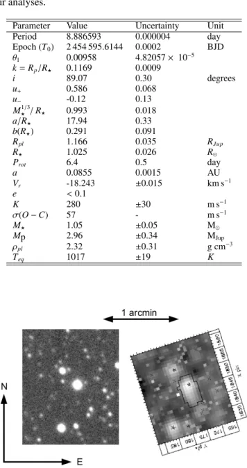
Fig. 3. The sky area around CoRoT-6 (brightest star near the cen-tre). Left: R-filter image with a resolution of ∼200taken with the
Euler 1.2m telescope. Right: Image taken by CoRoT, at the same scale and orientation. The jagged outline in its centre is the pho-tometric aperture mask used for this object; indicated are also CoRoT’s x and y image coordinates and positions of nearby stars from the Exo-Dat (Deleuil et al. 2009) database.
nate’ the light curve obtained when integrating within a pre-set photometric mask. To exclude the possibility of spurious vari-ation caused by such a contaminating object a comprehensive photometric (Deeg et al. 2009) and spectroscopic ground-based follow-up program is required.
The follow-up program initially consisted of observations with the radial velocity spectrograph SOPHIE (Bouchy et al. 2009; Perruchot et al. 2008), and photometric observations car-ried out at both the 0.46m telescope at the Wise observatory in Israel and the 1.2m Leonard Euler telescope at La Silla, Chile. These observations were initiated as soon as possible after
Fig. 4. Light curves of CoRoT-6 from ground-based photo-metric follow-up, given in normalized flux. The squares are sparse-coverage on-off photometry from the Euler telescope; the crosses are observations of an egress from WISE. They are plot-ted against the orbital phase; the vertical lines indicate the phase of first and last contact. The data clearly show that the transit is on the target star
Fig. 5. The phase-folded light curve of the CoRoT-6b. The mean errorbars in this plot have been calculated as the dispersion in all the points inside the bin and divided by the square root of the number of events within each bin. The median bin size is 12.9s and the resulting errorbars are 485 ppm. The dispersion inthe points outside transit is slightly higher, 500 ppm, revealing uncorrected red noise in the light curve at a low level.
CoRoT-6b had been identified as an exoplanetary candidate by the alarm mode.
3.1. Photometric observations
As mentioned above, the PSF of CoRoT is relatively large and covers typically 2000× 1000on the sky. The aperture mask used to calculate the flux from the target star needs to cover all or most of the PSF (or spacecraft jitter would introduce a periodic signal
Fig. 6. The χ2map of a trapezoid fit with the same parameters as the transit, in the moments of expected secondary transit. A 3σ upper limit of 1.8 × 10⁻⁴to the depth of the secondary transit can
be given from this plot.
and lower the precision of the actual photometry). The aperture mask will then have a significant probability of containing one or more fainter stars (see Fig. 3). The flux from these objects will thus contaminate the light curve from the target – and any vari-ation will produce a false signal in the required data. The light curve acquired by CoRoT and believed to be the result of an tran-siting planet can thus instead be the result of e.g., a background eclipsing star. Using the ephemeris for transits derived from the light curve of CoRoT, observations in and outside transit were scheduled and carried out at the Euler telescope on the nights of 8-10 July, 2008, and at the Wise observatory on 23 August, 2008. In both observations, part of the transit was observed to take place on CoRoT-6, at the right time and with the right depth at mid-transit (Fig 4). The target was thus verified as the ori-gin of the transit. Since the activity of CoRoT-6 is similar to the amplitude of the transit signal, and the timescale is similar, like-wise, this investigation proves that the activity is produced by the target.
3.2. Radial velocity observations
We acquired 14 spectra of the host star CoRoT-6 between late-June and early-September, 2008, in good weather conditions and with no strong moonlight contamination (see Table 3), at different orbital phases according to the ephemeris derived from the CoRoT photometry. These observations were per-formed with the SOPHIE instrument at the 1.93-m telescope of Haute-Provence Observatory, France as part of the CoRoT spec-troscopic follow-up (C. Moutou as PI). SOPHIE is a cross-dispersed, environmentally stabilized Echelle spectrograph ded-icated to high-precision radial velocity measurements (Bouchy & The Sophie Team 2006; Perruchot et al. 2008; Bouchy et al. 2009). To increase the throughput and reduce the read-out noise for this faint target, we used the high-efficiency mode (resolu-tion power R= 40, 000) of the spectrograph and the slow read-out mode of the 4096 × 2048 15-µm-pixel CCD detector. The two optical-fiber apertures were used, the first one centred on
the target and the second one on the sky. This second aperture, positioned 20away from the first one, was used to estimate the
spectral pollution caused by the sky background and the moon-light, which can be quite significant in these 3”-wide circular apertures – especially for faint targets. Exposures of a thorium-argon lamp were performed every 2-3 hours during each observ-ing night. They typically show drifts of around ∼ 3 m s−1, which is negligible compared to the photon noise, which is of the order of several tens m s−1.
Table 3. Radial velocities of CoRoT-6b measured with SOPHIE. BJD RV ±1 σ exp. time S/N p. pix. 2 454 000 (km s−1) (km s−1) (sec) (at 550 nm) 642.5591 -18.465 0.066 2400 16.8 646.4820 -17.967 0.039 1805 20.5 679.4155 -18.345 0.044 1698 20.1 681.4542 -17.999 0.048 2695 19.0 685.3983 -18.510 0.050 1792 21.0 689.4129 -18.202 0.063 3600 26.4 700.3532 -18.011 0.048 2002 21.6 702.3841 -18.333 0.072 3600 13.4 704.3410 -18.469 0.044 2436 21.1 706.3593 -18.229 0.041 2400 22.1 707.3968 -18.041 0.040 2400 21.3 711.3270 -18.341 0.049 2224 18.1 712.3234 -18.525 0.060 2400 16.8 715.4002 -18.321 0.059 2974 15.3
The spectra extraction and the radial velocity measurements were performed using the SOPHIE pipeline. Following the tech-niques described by Baranne et al. (1996) and Pepe et al. (2002), the radial velocities were measured from a weighted cross-correlation of the spectra with a numerical mask. We used a standard F0 mask that includes more than 3300 lines; cross-correlations with G2 and K5 masks gave similar results. The resulting cross-correlation functions (CCFs) were fitted by Gaussians to determine the radial velocities and the associated photon-noise errors. The full width at half maximum of those Gaussians is 13.6 ± 0.2 km s−1and its contrast is 10.4 ± 1.3 % of
the continuum.
Three of the 14 spectra show significant signal in the sky-background fiber, because of moonlight. This contamination was removed from CoRoT-6 spectra following the method de-scribed in Pollacco et al. (2008), Barge et al. (2008), and H´ebrard et al. (2008). This induces a significant radial velocity cor-rection for only one measurement: −400 ± 50 m s−1 at BJD= 2 454 689.4129.
The final radial velocity measurements are given in Table 3. They are displayed in Figs. 7 and 8, along with their Keplerian fit, using the orbital period and the transit central time derived from the CoRoT photometry. The derived orbital parameters are reported in Table 2, including errorbars computed from χ2 varia-tions and Monte Carlo experiments. Teqis the zero albedo
equi-librium temperature, with isotropic reemission f=1/4, and b(R?) being the impact parameter. The orbit was assumed to be circu-lar, which is a reasonable assumption for hot Jupiters. Fits with free eccentricities provide the limit e < 0.1, without significant improvement to the dispersion in the residuals nor significant effect on the other parameters of the orbit. Two measurements were performed close to the phase φ= 0, but after the end of the 4-hour duration transit; they should thus not be affected by the Rossiter-McLaughlin anomaly, as in for instance Bouchy et al. (2008).
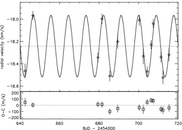
Fig. 7. Top: Radial velocity SOPHIE measurements of CoRoT-6 as a function of time, and Keplerian fit to the data. The or-bital parameters corresponding to this fit are reported in Table 2. Bottom:Residuals of the fit with 1-σ errorbars.
Fig. 8. Top: Phase-folded radial velocity SOPHIE measurements of CoRoT-6 as a function of the orbital phase, and Keplerian fit to the data. Orbital parameters corresponding to this fit are reported in Table 2. Bottom: Residuals of the fit with 1-σ errorbars.
The standard deviation of the residuals to the fit is σ(O−C)= 57 m s−1, implying a χ2of 18.8 for 12 degrees of freedom. This is slightly higher than expected, but remains in agreement with the expected errors in individual measurements, which range from ±39 to ±72 m s−1(see Table 3). Marginal structures are seen in
the residuals of the fits on timescales similar to the orbital pe-riod of CoRoT-6b (bottom panels of Figs. 7 and 8). They could at least be partially due to stellar activity, as the CoRoT photom-etry exhibits a (rotational) modulation of period 6.4 ± 0.5 days (see Sect.2.2). The SOPHIE coadded spectrum is of insufficient S/N in the wavelength region encompassing the Ca II H&K lines (S/N ∼ 6), so we cannot use this activity indicator. A check of the CCF bisector could reveal stellar activity or a blend with a binary as the main cause of the radial velocity variations. This check does not, however, uncover any significant dispersion in
the bisector nor any trend of it changing as a function of ra-dial velocity (see Fig. 9, upper panel). The residuals of the fits do not either show significant anti-correlation with the bisectors (Fig. 9, lower panel), as could be expected in cases of stellar activity. This is however at the limit of our detection. These anti-correlations have allowed in some cases a subtraction of the ra-dial velocity jitter due to stellar activity (see, e.g., Melo et al. (2007); Boisse et al. (2009)), which is not possible here because of the large errorbars. The standard deviation in the bisectors is σ = 94 m s−1, i.e., about two times the size of the residuals. This
agrees with the errorbars of the bisectors, which are two times larger than the error in the radial velocities.
Keplerian fits to the radial velocity measurements with free period and phase infer parameters that are in agreement with the CoRoT ephemeris, with , however, larger errorbars in these two parameters. The dispersion in the residuals could in that case decrease to 40 m s−1, which is slightly too low according to the errorbars in individual radial velocities.
We can thus conclude that the transit-signal detected in the CoRoT light curve could be caused by a massive planet or-biting the star. The planet CoRoT-6b induces a radial velocity oscillation of its host star with a semi-amplitude K = 280 ± 30 m s−1, in agreement with the photometric phase and period, P= 8.88 days.
Fig. 9. Bisector span as a function of the radial velocity (top) and the radial velocity residuals after the Keplerian fit (bottom). No significant dispersion nor trend, which would have indicated activity or blend, is detected.
Table 4. Observing log of dates and integration times of the VLT/UVES spectra.
Date Integration time (s) 2008-08-27T02:43:07.087 2380
2008-08-27T03:23:35.587 2380 2008-09-01T00:03:51.99 2380 2008-09-01T00:44:20.386 2380
3.3. Low resolution spectroscopy and spectral type classification
To derive the spectral type of CoRoT 6 and obtain prelimi-nary values of its physical parameters, we observed the tar-get star with the low-resolution (LR) spectrograph mounted at the Nasmyth focus of the 2m Alfred Jensch telescope of the Th¨uringer Landessternwarte Tautenburg (TLS). Two LR spec-tra covering the wavelength range 4950 − 7320 Å at a resolving power R ≈ 2100 were taken on August the 3rd and 4th, 2008, under good and clear sky conditions. During each night, three consecutive exposures of 20 minutes were acquired to remove cosmic ray hits leading to a final S /N ≈ 80 for each coadded spectrum. The spectral type of CoRoT 6 was derived by com-paring the LR spectra of the target with a suitable grid of stellar templates, as described in Frasca et al. (2003) and Gandolfi et al. (2008). The method has proven to be quite reliable when de-riving stellar temperature within one spectral subclass, pressure (or luminosity) within one class, and metallicity within 0.3 – 0.5 dex. In the case of CoRoT-6, we derive a spectral type of F9, a luminosity class of V, and a low metallicity (see method 5 in Table 6).
3.4. High resolution spectroscopy and stellar analysis Because of the faintness of CoRoT-6, the SOPHIE spectra de-scribed in the last section cannot be used to carry out the stellar modeling and thus determine the fundamental physical param-eters of the host star to the required precision. One stellar pa-rameter, the stellar density, can under ideal circumstances be ob-tained from a transit light curve of sufficient photometric preci-sion (e.g., Seager & Mall´en-Ornelas 2003). Nevertheless, high-precision photometric and spectroscopic measurements carried out on other exo-planetary host stars, suggest that this rarely in-fers reliably to the other properties of the star – mainly because of flaws in stellar theory (Winn et al. 2008). We have therefore scheduled regular observations with the UVES spectrograph on ESO’s Very Large Telescope (8.2m) VLT to constrain the re-quired parameters more accurately. We obtained four exposures each of 2380 s, using a slit width of 000
·8, which yields a
resolv-ing power of ∼ 65 000 (Table 4, ESO Program Identifier 081.C-0413(C)). The signal-to-noise ratio is ∼ 100 over the entire range of wavelengths used in the modeling. As is now standard practice in the analysis of CoRoT stars, we use several different meth-ods to model the stellar spectra in terms of fundamental physical parameters. Each method is applied by different teams indepen-dently.
One method uses the Spectroscopy Made Easy (SME 2.1) package (Valenti & Piskunov 1996; Valenti & Fischer 2005), which uses a grid of stellar models (Kurucz models or MARCS models – see below) to determine the fundamental stellar param-eters iteratively. This is achieved by fitting the observed spec-trum directly to the synthesized specspec-trum and minimizing the discrepancies using a non-linear least-squares algorithm. In
ad-dition, SME utilises input from the VALD database (Kupka et al. 1999; Piskunov et al. 1995) . The uncertainties using SME, as found by Valenti & Fischer (2005), and based on a large sam-ple (of more than 1000 stars) are 44K in Teff, 0.06 dex in log g,
and 0.03 dex in [M/H] per measurement. However, by compar-ing the measurements with model isochrones they found a larger, systematic offset of ∼ 0.1 dex and a scatter that can occasionally reach 0.3 dex, in log g. In CoRoT-6, we find an internal discrep-ancy using SME of 0.1 dex depending on which ion we use to determine log g. We therefore assign 0.1 dex as our 1 σ preci-sion.
The second method used by us is based on the semi-automatic package VWA (Bruntt et al. 2008), which performs iterative fitting of synthetic spectra to reasonably isolated spec-tral lines. This method constrain Teff, log g, and [Fe/H] to about
120 K, 0.13 dex, and 0.09 dex, respectively, including estimated uncertainties in the applied model atmospheres. However, larger deviations can occur for special cases when using this method (Bruntt et al. 2008).
A third method uses specific, individual models, e.g., those of Kurucz (1993) to model the Hα line and the MARCS model grid (Gustafsson et al. 2008) for the other ionic species. It uses special software to reproduce the line profiles, calculating the stellar parameters (e.g., the gravity is calculated from the [Mg i] and [Na i] line wings). It thus does not specifically perform an iterative fitting on a grid of models. This method is described in detail in Barge et al. (2008).
A fourth scheme again utilises the equivalent width of a set of lines of different elements, calculating ratios. The equivalent width (EW) of spectral lines varies as a function of tempera-ture and can therefore be used to measure stellar temperatempera-tures (Teff). Using ratios of spectral lines obviates the dependency
of single lines on instrumental or rotational broadening. Each temperature-calibrated line ratios can be used to derive an indi-vidual measurement of the stellar temperature Teff. The
preci-sion in the combined temperature is improved by a factor √N, where N is the number of independent measurements (Aigrain et al. 2009). The description of the calibration set of equivalent-width line-ratios that we use here can be found in Sousa et al. (2009). The calibration consists of 433 equivalent-width line-ratios (composed of 171 spectral lines of different chemical el-ements) calibrated in temperature with the sample of FGK stars presented in Sousa et al. (2008). This technique is automated to produce from the input stellar spectra the derivation of the stel-lar temperature, the equivalent width measurements being per-formed with the ARES software (Sousa et al. 2007) and the stellar temperature being derived using the calibrated line ra-tios. This technique provides a model-independent stellar spec-troscopic temperature. The spectra of CoRoT-6 used here is the same as that presented earlier in Sect. 3.4. Of the 433 line-ratios, 173 line-ratios were measured and kept to derive the stellar tem-perature; the other line ratios were either not measured because at least one of the spectral lines was not measurable or were dis-regarded because the derived Teffwas more than 2σ away from
the average Teff for all the line-ratios (because for example a
failure of the accurate automated measurement of the equivalent width of one of the lines). When combining the 173 measure-ments of temperature, the stellar effective temperature obtained is Teff= 6006±73K. This value is lower than the others in Table
6, but consistent within the errorbars.
All the methods (both low-dispersion and high-dispersion spectroscopy) utilized here allow a determination of the metal-licity and we find consistent results (see Table 6). Concerning the abundances of metals, the most detailed method, however, is the
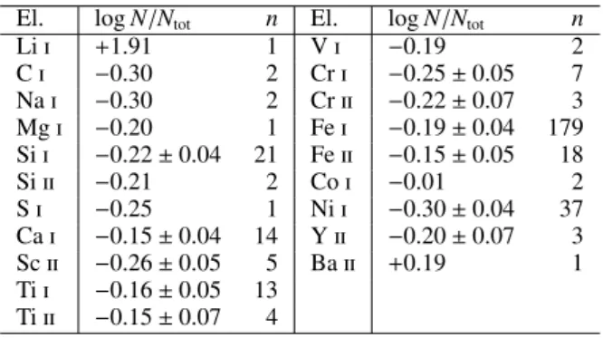
Table 5. Abundance pattern in CoRoT-6 for 16 elements. El. log N/Ntot n El. log N/Ntot n
Li i +1.91 1 V i −0.19 2 C i −0.30 2 Cr i −0.25 ± 0.05 7 Na i −0.30 2 Cr ii −0.22 ± 0.07 3 Mg i −0.20 1 Fe i −0.19 ± 0.04 179 Si i −0.22 ± 0.04 21 Fe ii −0.15 ± 0.05 18 Si ii −0.21 2 Co i −0.01 2 S i −0.25 1 Ni i −0.30 ± 0.04 37 Ca i −0.15 ± 0.04 14 Y ii −0.20 ± 0.07 3 Sc ii −0.26 ± 0.05 5 Ba ii +0.19 1 Ti i −0.16 ± 0.05 13 Ti ii −0.15 ± 0.07 4
VWA method (Bruntt et al. 2008), and the results can be found in Table 5 and Fig. 10. The listed uncertainties in Table 5 include the uncertainty on the atmospheric parameters (0.04 dex) and the uncertainty on the mean value (> 3 lines).
Fig. 10. Relative abundances derived from modelling the VLT/UVES and utilising the VWA package. Error bars are 1 σ.
The results of our analysis of CoRoT-6 can be found in Table 6. In the case of this star, all 5 methods mentioned above have been evaluated (low- and high-resolution spectroscopy). The fact that we use several different methods to derive the fun-damental stellar parameters in general, as well as the log g in particular, and reach consistent results within the applicable er-rors is highly satisfying.
4. Discussion and conclusion
4.1. Stellar Parameters
To derive the mass and radius of the parent star, we use the same methodology applied to earlier CoRoT planets (e.g., Barge et al. 2008; Bouchy et al. 2008). The light curve analysis provides M1/3/R
?. It is usually because this measurable provides a more
robust estimate of the stellar fundamental parameters. In the case of CoRoT-6, however, we have both very good spectral informa-tion from UVES, as well as the excellent CoRoT light curve. We find that the fundamental values agree reasonably well. As dis-cerned from the spectral analysis (Table 6), the stellar parameters are consistent with a spectral type of F9V, an effective tempera-ture of about 6090 ± 50K, a gravity compatible with a dwarf star, and a low metallicity of −0.20 (see also Table 5). From the light curve, we derive a M1/3/R
?of 0.993 ± 0.018. Then by using the
values for M1/3/R?from the light curve and Teffand metallicity
from the spectral analysis (using STAREVOL – see Sect. 4.3), we deduce a stellar mass of 1.05 ± 0.05M and a stellar radius of
Fig. 11. The Li abundance as a function of (B − V)0. The
red marker with errorbars represents the litium abundance of CoRoT-6. The Li I equivalenth widths for Pleiades stars (Soderblom et al. 1993a) are plotted with plus symbols.
1.025 ± 0.026R . Using this radius yields a log g from the light
curve values of 4.44 ± 0.023, while the value derived from the [Ca i] , [Na i] , and [Mg i] line wings in the Echelle spectrum is 4.43 ± 0.1 (from SME).
The metallicity of the star is quite low, ∼ −0.20 dex. While it is generally considered that exoplanets orbit stars with metal-licities greater than the one of the Sun, (Santos et al. 2003), this has been found in the very large sample of stars selected for ra-dial velocity studies. In the sample of planets found in transit studies, however, ∼30% of the 53 stars for which metallicity has been published in the The Extrasolar Planets Encyclopedia cata-log1are under-abundant in metals. In a larger study, Ammler-von Eiff et al. (2009) included a consistent re-observation and anal-ysis of 13 transiting hosts, as well as a re-analanal-ysis of about 40 other objects (including CoRoT-1b, CoRoT-2b, CoRoT-3b, and CoRoT-4b), come to similar conclusions as Santos et al. (2004), i.e., that the presence of planets is a strongly rising function of metallicity. We note, however, that even in the data of Ammler-von Eiff et al. (2009), about 20% of the stars are under-abundant. As pointed out by these authors, there is probably a difference in planetary structure that depends on the metallicity of the star and reflects different formation mechanisms. We point out here that in the case of CoRoT-6b the planet is very much similar to other previously classified ‘hot Jupiter’s’.
4.2. Planetary parameters
There is no ambiguity in the determination of the stellar ra-dius and thus the planetary rara-dius is well constrained to Rp =
1.166 ± 0.035 RJup. Taking into account the semi-amplitude of
the radial velocity curve K= 280 ± 30 m s−1and the orbit
incli-nation derived from the transit i= 89◦
·07±0◦·33, the stellar mass
of M? = 1.05 ± 0.05 M translates into a planetary mass of
2.96 ± 0.34 MJupfor CoRoT-6b. The planetary average density,
ρpl, is 2.32 g cm−3.
Comparing this latter parameter with the values for the other giant exoplanets found by CoRoT (and thus excluding CoRoT-7b) and for which we have very well determined values of ρpl,
we find that the planets divide into 3 groups. In the brown dwarf mass regime, CoRoT-3b, has a very high average density of 26.4 g cm−3 demonstrating its (near) stellar status (Deleuil
et al. 2008). CoRoT-1b, CoRoT-4b, and CoRoT-5b all have 0.2 < ρpl < 0.5 g cm−3. These planets also have a mass of 0.47
< Mpl < 1.03MJup (Barge et al. 2008; Aigrain et al. 2008;
Rauer et al. 2009). The third group consisting of CoRoT-2b and CoRoT-6b have ρplof 1.3 and 2.32 g cm−3, respectively (Alonso
et al. 2008). Both of these last set of planets have masses of ∼ 3MJup
The period of the planet orbiting CoRoT-6 is 8.9 days, which makes CoRoT-6b one of the (so far rare) transiting planets with a relatively long period (P ≥ 5 days). To date, only 2 of the 62 known transiting planets have periods longer then CoRoT-6b and only 6 planets have periods ≥ 5 days, 2 of which were discovered by CoRoT. Other known transiting objects with long periods are WASP-8b with P = 8.16 days, M = 2.23 MJup (Smith et al.
2009), CoRoT-4b with P= 9.20 days, M = 0.72 MJup(Aigrain
et al. 2008), and HD 17156b with P = 21.22 days, M = 3.21 MJup, (Barbieri et al. 2007; Fischer et al. 2007). There
is also the case of HD 80606b with P = 111.43 days, M = 3.94 MJup (Naef et al. 2001). Thus, of the 5 transiting objects
with periods longer than 8 days, 4 have masses of between 2 and 4 MJup, and only one – CoRoT-4b– is a somewhat smaller
ob-ject of M = 0.72 MJup. For the objects with periods between 4
and 8 days, on the other hands, 6 have masses below one MJup, 3
are larger, while one is the planet-brown dwarf boundary object CoRoT-3b (Deleuil et al. 2008). Of the 3 objects more massive than 1 MJup, one barely makes the grade, another has only an
up-per limit to its mass and the third is more massive than 9 MJup.
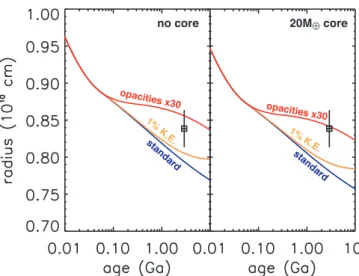
The period derived from the the CoRoT light curve is fully in phase with that derived from the radial velocity measure-ments. The bootstrap analysis described in Sect. 2.2 is consis-tent with the eccentricity of the planetary orbit being ≤ 0.1, as derived from an analysis of the radial velocity curve (Sect. 3.2). While circularisation of planetary orbits may take quite some time (Jackson et al. 2008), we note that the age of the CoRoT-6b system derived below is consistent with a low value to the ec-centricity at the distance of 0.08 AU. We used the evolutionary models of Guillot (2008) to investigate whether a planet with a relatively longer period (and thus less incident radiation) would behave differently from a more ‘classical’ hot Jupiter. As can be seen from the results in Fig. 12, it does not. It is also a modestly inflated planet requiring: (1) a low core mass, consistent with the low-metallicity of the parent star and the star-planet metal-licity correlation; and (2) either some tidal dissipation (equiv-alent to a few % of the incoming stellar heat flux) or an order of magnitude higher interior opacity than is generally assumed. To estimate the expected thermal evaporation of CoRoT-6b, we applied the method described in Lammer et al. (2009) and ob-tained mass loss rates given by dMdt ∼ 2 × 10⁻⁸g s−1that are
about a factor 100 lower than the loss rate of HD209458b (Yelle 2006; Penz et al. 2008). The low mass-loss rate of CoRoT-6b rel-ative to other hot gas giants is caused by the high density of the planet and its larger orbital separation (0.08 AU). Furthermore, because of this high density, we expect the stellar EUV-induced dynamical expansion of the upper atmosphere of CoRoT-6b not to be as efficient as that of lower density close-in gas giants, hence adiabatic cooling should be less efficient. This means that a hot thermosphere-exosphere containing mainly ionized hydro-gen atoms is expected. This strong ionization would enhance the
opacities x30 opacities x30 1% K.E. 1% K. E. standard standard no core 20M⊕ core
Fig. 12. Theoretical models for the contraction of CoRoT-6b with time compared to the observations. The models (Guillot 2008) assume either solar composition and no core (left panel) or the presence of a central dense core of (right panel). In each case, three possible evolution models are shown: (1) a standard model; (2) a model assuming that 1% of the incoming stellar luminosity is transformed into kinetic energy and dissipated in the deep interior by tides; (3) a model in which interior opacities have been arbitrarily increased by a factor 30.
planet’s ability to protect itself against stellar wind erosion even in the absence of a strong planetary magnetic field (Lammer et al. 2009). Therefore, we can expect that the mass of CoRoT-6b has not changed significantly since its origin.
4.3. Evolutionary state of the star: activity, rotation, and7Li
abundance
CoRoT-6 appears to be a solar-like star but clearly exhibits more activity, based on its light curve. It displays more rapid rota-tion and thus could be younger than our Sun. Unfortunately, our UVES spectrum did not cover the [Ca ii] lines, although our SOPHIE data covers this wavelength region, albeit at much lower S/N. In spite of the very agitated state of the star discerned from photometry, we see, however, no indication of activity in the SOPHIE data. The v sin i is 7.5±1 km s−1, which indicates that the star rotates ∼ 4-5 times more rapidly than the Sun. The 2-3 % amplitude of the rotation-modulated light curve suggests that the surface coverage by photospheric spots on CoRoT-6 is significantly higher than on the Sun. This high level of magnetic activity is most likely to be linked to its rapid rotation. High activity and rapid rotation are considered to be signs of stellar youth (Simon et al. 1985; Guedel et al. 1997; Soderblom et al. 2001) because both rotation and magnetic activity in late-type dwarfs continue to decrease as the star evolves unless the star’s rotation is tidally locked in a close binary system. It has also been suggested by e.g., Skumanich (1972) that the Li surface abun-dance decreases with stellar evolution. Hence, another index of stellar youth is provided by the Li I absorption line of 75 mÅ equivalent width that we detected in the spectrum of CoRoT-6, indicating a7Li abundance (log N/Ntot) of+1.91 (Table 5).
Based on the Li abundance for the appropriate type of star and the results of Sestito & Randich (2005), we estimate the age of CoRoT-6 to be between 2.5 and 4.0 Gyr. It is however worth noting that solar-type stars reach the zero-age main se-quence (ZAMS) rotating at a variety of rates, from roughly solar on up to 100 times that velocity, as seen, for example, in the Pleiades (Stauffer & Hartmann 1987; Soderblom et al. 1993b,a). A wide range of Li abundances are also found in the Pleiades, and data for CoRoT-6 can actually be included into the range of Li-values found for that cluster, although all other indications are that the CoRoT-6 is significantly older than the Pleiades (see Fig. 11). Li depletion has also been found in several T Tauri stars at levels inconsistent with their young ages (Magazzu et al. 1992). Hence, while magnetic activity, rapid rotation, and ele-vated Li abundance may be signs of stellar youth, the converse is not necessarily true. Furthermore, stars of lower metallicity have a shallower outer convection zone. This means that lithium lasts longer in these stars, mainly because the distance between the convection zone and the nuclear destruction region is larger (Castro et al. 2009). In the case of CoRoT-6, the high7Li
abun-dance could be explained by the low metallicity, even in a rel-atively mature star. This should also be viewed in terms of the results of Israelian et al. (2009), who determined a relation be-tween the presence of planets and an under-abundance of7Li,
the explanation being that the presence of a planet could increase the amount of mixing and deepen the convective zone to such an extent that the Li can be burned. In the case of CoRoT-6, the planet is relatively far away and it could thus be that the effect is negligible in this case.
We have also used evolutionary models of STAREVOL (Palacios, private communication) and CESAM (Morel & Lebreton 2008), and using the M1/3/R?relation and stellar ra-dius of 1.02R (Table 2 - see above) to calculate the age of
CoRoT-6, obtaining a value between 1 and 3.3 Gyr. Combining this value with the7Li analysis above would restrict the age to a
range between 2.5 and 3.3 Gyr. In view of the rapid rotation and large level of activity, we would be inclined to favor the lower value but there is no information in our data that requires this.
5. Summary
The CoRoT space mission has discovered its sixth transiting planet, designated CoRoT-6b. In summary, we conclude that:
– A planet of 2.96 MJuporbits the star CoRoT 0106017681.
– Its orbital period is ∼8.9 days and the ephemeris for the tran-sits is compatible with a circular orbit (e ≤ 0.1). The planets radius is 1.166 RJup.
– CoRoT-6b has a density of 2.32 g cm−3, similar to that of 2b but higher than the lower mass objects CoRoT-1b, CoRoT-4b, and CoRoT-5b.
– The star is solar-like with a spectral type of F9V, a mass of 1.05 M , and a stellar radius of 1.025 R . Its metallicity is
relatively low (−0.20 dex) compared to other planet-hosting stars.
– We assign an age of 1-3.3 Gyrs, based on evolutionary tracks. The higher end of this range is consistent with the high
7Li abundance, given the paucity of other metals.
– No secondary eclipse is observed in the CoRoT data. This is consistent with expectations, becasue of the greater distance from the star in this case than for e.g., either CoRoT-1b and CoRoT-2b.
– The discovery of CoRoT-6b clearly demonstrates the capa-bility of CoRoT to discover and study long-period transiting planets.
Acknowledgements. We are grateful to N. Piskunov of Uppsala Astronomical Observatory for making SME available to us, and for answering questions about its implementation and operation.
The team at IAC acknowledges support by grant ESP2007-65480-C02-02 of the Spanish Ministerio de Ciencia e Innovaci´on.
The building of the input CoRoT/Exoplanet catalog (Exo-dat) was made possible thanks to observations collected for years at the Isaac Newton Telescope (INT), operated on the island of La Palma by the Isaac Newton group in the Spanish Observatorio del Roque de Los Muchachos of the Instituto de Astrosica de Canarias.
The German CoRoT team (TLS and University of Cologne) acknowledges DLR grants 50OW0204, 50OW0603, and 50QP07011.
We are also grateful to an anonymous referee whose very constructive com-ments have helped us produce a more stringent paper.
References
Aigrain, S., Collier Cameron, A., Ollivier, M., et al. 2008, A&A, 488, L43 Aigrain, S. & Irwin, M. 2004, MNRAS, 350, 331
Aigrain, S., Pont, F., Fressin, F., et al. 2009, A&A, 506, 425 Alapini, A. & Aigrain, S. 2009, MNRAS, 397, 1591
Alonso, R., Aigrain, S., Pont, F., Mazeh, T., & The CoRoT Exoplanet Science Team. 2009, in IAU Symposium, Vol. 253, IAU Symposium, 91–96 Alonso, R., Auvergne, M., Baglin, A., et al. 2008, A&A, 482, L21
Ammler-von Eiff, M., Santos, N. C., Sousa, S. G., et al. 2009, A&A, 507, 523 Auvergne, M., Bodin, P., Boisnard, L., et al. 2009, A&A, 506, 411
Baglin, A., Michel, E., Auvergne, M., & The COROT Team. 2006, in ESA Special Publication, Vol. 624, Proceedings of SOHO 18/GONG 2006/HELAS I, Beyond the spherical Sun
Baranne, A., Queloz, D., Mayor, M., et al. 1996, A&AS, 119, 373 Barbieri, M., Alonso, R., Laughlin, G., et al. 2007, A&A, 476, L13 Barge, P., Baglin, A., Auvergne, M., et al. 2008, A&A, 482, L17
Boisnard, L. & Auvergne, M. 2006, in ESA Special Publication, Vol. 1306, ESA Special Publication, ed. M. Fridlund, A. Baglin, J. Lochard, & L. Conroy, 19–+
Boisse, I., Moutou, C., Vidal-Madjar, A., et al. 2009, A&A, 495, 959 Bonomo, A. S., Aigrain, S., Bord´e, P., & Lanza, A. F. 2009, A&A, 495, 647 Bouchy, F., H´ebrard, G., Udry, S., et al. 2009, A&A, 505, 853
Bouchy, F., Queloz, D., Deleuil, M., et al. 2008, A&A, 482, L25
Bouchy, F. & The Sophie Team. 2006, in Tenth Anniversary of 51 Peg-b: Status of and prospects for hot Jupiter studies, ed. L. Arnold, F. Bouchy, & C. Moutou, 319–325
Bruntt, H., De Cat, P., & Aerts, C. 2008, A&A, 478, 487
Castro, M., Vauclair, S., Richard, O., & Santos, N. C. 2009, A&A, 494, 663 Christian, D. J., Gibson, N. P., Simpson, E. K., et al. 2009, MNRAS, 392, 1585 Deeg, H. J., Gillon, M., Shporer, A., et al. 2009, A&A, 506, 343
Deleuil, M., Deeg, H. J., Alonso, R., et al. 2008, A&A, 491, 889 Deleuil, M., Meunier, J. C., Moutou, C., et al. 2009, AJ, 138, 649 Fischer, D. A., Vogt, S. S., Marcy, G. W., et al. 2007, ApJ, 669, 1336 Frasca, A., Alcal´a, J. M., Covino, E., et al. 2003, A&A, 405, 149 Gandolfi, D., Alcal´a, J. M., Leccia, S., et al. 2008, ApJ, 687, 1303 Geem, Z. W., Kim, J. H., & Lonatathan, G. V. 2001, Simulation, 76, 60 Gim´enez, A. 2006, A&A, 450, 1231
Guedel, M., Guinan, E. F., & Skinner, S. L. 1997, ApJ, 483, 947 Guillot, T. 2008, Physica Scripta Volume T, 130, 014023
Gustafsson, B., Edvardsson, B., Eriksson, K., et al. 2008, A&A, 486, 951 H´ebrard, G., Bouchy, F., Pont, F., et al. 2008, A&A, 488, 763
Israelian, G., Delgado Mena, E., Santos, N. C., et al. 2009, Nature, 462, 189 Jackson, B., Greenberg, R., & Barnes, R. 2008, ApJ, 678, 1396
Kupka, F., Piskunov, N., Ryabchikova, T. A., Stempels, H. C., & Weiss, W. W. 1999, A&AS, 138, 119
Kurucz, R. 1993, SYNTHE Spectrum Synthesis Programs and Line Data. Kurucz CD-ROM No. 18. Cambridge, Mass.: Smithsonian Astrophysical Observatory, 1993., 18
Lammer, H., Odert, P., Leitzinger, M., et al. 2009, A&A, 506, 399 L´eger, A., Rouan, D., Schneider, J., et al. 2009, A&A, 506, 287 Magazzu, A., Rebolo, R., & Pavlenko, I. V. 1992, ApJ, 392, 159 Mandel, K. & Agol, E. 2002, ApJ, 580, L171
Markwardt, C. B. 2009, in Astronomical Society of the Pacific Conference Series, Vol. 411, Astronomical Society of the Pacific Conference Series, ed. D. A. Bohlender, D. Durand, & P. Dowler, 251–+
Melo, C., Santos, N. C., Gieren, W., et al. 2007, A&A, 467, 721 Morel, P. & Lebreton, Y. 2008, Ap&SS, 316, 61
Moutou, C., Bruntt, H., Guillot, T., et al. 2008, A&A, 488, L47 Naef, D., Latham, D. W., Mayor, M., et al. 2001, A&A, 375, L27
Penz, T., Erkaev, N. V., Kulikov, Y. N., et al. 2008, Planet. Space Sci., 56, 1260 Pepe, F., Mayor, M., Galland, F., et al. 2002, A&A, 388, 632
Perruchot, S., Kohler, D., Bouchy, F., et al. 2008, in Society of Photo-Optical Instrumentation Engineers (SPIE) Conference Series, Vol. 7014, Society of Photo-Optical Instrumentation Engineers (SPIE) Conference Series Piskunov, N. E., Kupka, F., Ryabchikova, T. A., Weiss, W. W., & Jeffery, C. S.
1995, A&AS, 112, 525
Pollacco, D., Skillen, I., Collier Cameron, A., et al. 2008, MNRAS, 385, 1576 Queloz, D., Bouchy, F., Moutou, C., et al. 2009, A&A, 506, 303
Quentin, C. G., Barge, P., Cautain, R., et al. 2006, in ESA Special Publication, Vol. 1306, ESA Special Publication, ed. M. Fridlund, A. Baglin, J. Lochard, & L. Conroy, 409–+
Rauer, H., Queloz, D., Csizmadia, S., et al. 2009, A&A, 506, 281 Santos, N. C., Israelian, G., & Mayor, M. 2004, A&A, 415, 1153
Santos, N. C., Israelian, G., Mayor, M., Rebolo, R., & Udry, S. 2003, A&A, 398, 363
Seager, S. & Mall´en-Ornelas, G. 2003, ApJ, 585, 1038 Sestito, P. & Randich, S. 2005, A&A, 442, 615
Simon, T., Herbig, G., & Boesgaard, A. M. 1985, ApJ, 293, 551 Skumanich, A. 1972, ApJ, 171, 565
Smith, A. M. S., Hebb, L., Collier Cameron, A., et al. 2009, MNRAS, 398, 1827 Soderblom, D. R., Jones, B. F., Balachandran, S., et al. 1993a, AJ, 106, 1059 Soderblom, D. R., Jones, B. F., & Fischer, D. 2001, ApJ, 563, 334
Soderblom, D. R., Stauffer, J. R., Hudon, J. D., & Jones, B. F. 1993b, ApJS, 85, 315
Sousa, S. G., Alapini, A., Israelian, G., & Santos, N. C. 2009, ArXiv e-prints Sousa, S. G., Santos, N. C., Israelian, G., Mayor, M., & Monteiro, M. J. P. F. G.
2007, A&A, 469, 783
Sousa, S. G., Santos, N. C., Mayor, M., et al. 2008, A&A, 487, 373 Stauffer, J. R. & Hartmann, L. W. 1987, ApJ, 318, 337
Surace, C., Alonso, R., Barge, P., et al. 2008, in Presented at the Society of Photo-Optical Instrumentation Engineers (SPIE) Conference, Vol. 7019, Society of Photo-Optical Instrumentation Engineers (SPIE) Conference Series Valenti, J. A. & Fischer, D. A. 2005, ApJS, 159, 141
Valenti, J. A. & Piskunov, N. 1996, A&AS, 118, 595
Winn, J. N., Holman, M. J., Torres, G., et al. 2008, ApJ, 683, 1076 Yelle, R. V. 2006, Icarus, 183, 508
1 Research and Scientific Support Department, European Space
Agency, Keplerlaan1, NL-2200AG, Noordwijk, The Netherlands e-mail: [email protected]
2 Institut d’Astrophysique de Paris, UMR7095 CNRS, Universit´e
Pierre & Marie Curie, 98bis boulevard Arago, 75014 Paris, France
3 LAM, UMR 6110, CNRS/Univ. de Provence, 38 rue F.
Joliot-Curie, 13388 Marseille, France
4 Institut d’Astrophysique Spatiale, Universite Paris XI, F-91405
Orsay, France
5 LESIA, Observatoire de Paris-Meudon, 5 place Jules Janssen,
92195 Meudon, France
6 School of Physics, University of Exeter, Exeter, EX4 4QL 7 Netherlands Institute for Space Research, SRON, Sorbonnelaan 2,
3584 CA, Utrecht, The Netherlands
8 Wise Observatory, Tel Aviv University, Tel Aviv 69978, Israel 9 Instituto de Astrof´ısica de Canarias , E-38205 La Laguna,
Tenerife, Spain
10 Th¨uringer Landessternwarte, 07778 Tautenburg, Germany 11 Institute of Planetary Research, DLR, 12489 Berlin, Germany 12 Rheinisches Institut f¨ur Umweltforschung an der Universit¨at zu
K¨oln, Aachener Strasse 209, 50931, K¨oln, Germany
13 Space Research Institute, Austrian Academy of Science,
Schmiedlstr. 6, A-8042 Graz, Austria
14 LUTH, Observatoire de Paris-Meudon, 5 place Jules Janssen,
92195 Meudon, France
15 Observatoire de Gen`eve, Universit´e de Gen`eve, 51 chemin des
Maillettes, 1290 Sauverny, Switzerland
16 Universit de Nice Sophia Antipolis, CNRS, Observatoire de la Cte
d’Azur, BP 4229, 06304 Nice, France
17 Observat´orio Nacional, Rio de Janeiro, RJ, Brazil
18 Institute for Astronomy, University of Vienna,
T¨urkenschanzstrasse 17, 1180, Vienna, Austria
19 IAG Universit´e du Li`ege, All´ee du 6 auˆot 17, Li`ege 1, Belgium 20 IAG Universidade de Sao Paulo, Sao Paulo, Brasil
21 TU Berlin, Zentrum f¨ur Astronomie und Astrophysik,
Hardenbergstr. 36, 10623 Berlin, Germany
22 Observatoire de Haute-Provence, CNRS/OAMP, 04870 St Michel
l’Observatoire, France
23 Dept. de Astrofsica, Universidad de La Laguna, Tenerife, Spain 24 Oxford Astrophysics, University of Oxford, Keble Road, Oxford
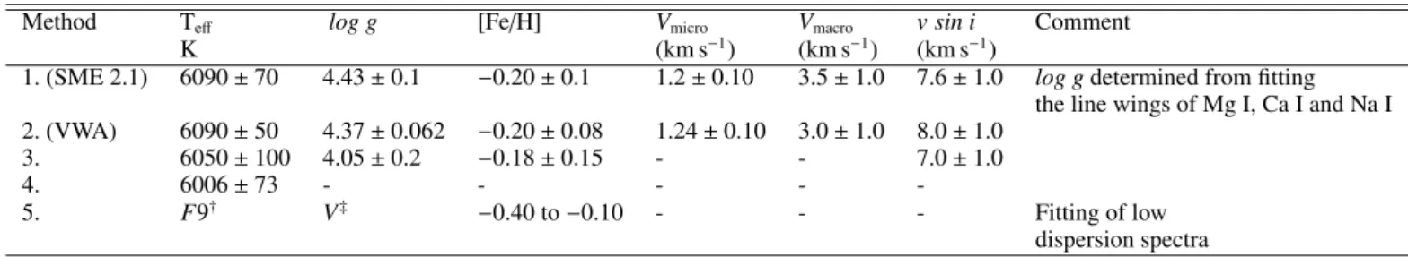
Table 6. Stellar parameters for CoRoT-6 derived through modeling spectra and using the 4 methods described in the text. The errors are 1 σ
Method Teff log g [Fe/H] Vmicro Vmacro v sin i Comment
K (km s−1) (km s−1) (km s−1)
1. (SME 2.1) 6090 ± 70 4.43 ± 0.1 −0.20 ± 0.1 1.2 ± 0.10 3.5 ± 1.0 7.6 ± 1.0 log gdetermined from fitting the line wings of Mg I, Ca I and Na I 2. (VWA) 6090 ± 50 4.37 ± 0.062 −0.20 ± 0.08 1.24 ± 0.10 3.0 ± 1.0 8.0 ± 1.0 3. 6050 ± 100 4.05 ± 0.2 −0.18 ± 0.15 - - 7.0 ± 1.0 4. 6006 ± 73 - - - - -5. F9† V‡ −0.40 to −0.10 - - - Fitting of low dispersion spectra †: spectral type from template fitting.